Exercise 3.2: Eye Pattern according to Gaussian Low-Pass

Basic transmission pulse $g_s(t)$ ⇒ blue curve,
basic detection pulse $g_d(t)$ ⇒ red curve

Let a binary bipolar redundancy-free baseband system with bit rate $R_{\rm B} = 100\,{\rm Mbit/s}$ be given. Further:

Rectangular transmission pulses, possible amplitude values $± 1\,{\rm V}$.

The AWGN noise power density $($on the resistor $1 \, \Omega)$: $N_0=10^{\rm -9} \, {\rm V}^2/{\rm Hz}$.

Receiver filter is a Gaussian low-pass with cutoff frequency $f_{\rm G} = 50 \, {\rm MHz}$. The frequency response is:

$$H_{\rm G}(f) = {\rm e}^{- \pi \hspace{0.05cm}\cdot \hspace{0.05cm}{f}^2/({2f_{\rm G}})^2} \hspace{0.05cm}.$$

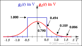
The basic detection pulse $g_d(t) = g_s(t) * h_{\rm G}(t)$ is shown in the graph (red curve).
Some prominent pulse sample values are indicated.

The detection noise power can be calculated using the following equation:

$$\sigma_d^2 = {N_0}/{2} \cdot \int_{-\infty}^{+\infty} |H_{\rm G}(f)|^2 \,{\rm d} f \hspace{0.05cm}.$$

The "eye diagram" can be used to determine the bit error probability $($in general: symbol error probability$)$.

The mean symbol error probability $p_{\rm S}$ is obtained from this after averaging over all possible noiseless detection samples in consideration of the noise rms value $\sigma_d$.
The worst-case error probability serves as an upper bound for $p_{\rm S}$:

$$p_{\rm U} = {\rm Q} \left( \frac{\ddot{o}(T_{\rm D})/2}{ \sigma_d} \right) \hspace{0.3cm}{\rm with}\hspace{0.3cm}\frac{\ddot{o}(T_{\rm D})}{ 2}= g_d(t=0) - |g_d(t=T)|- |g_d(t=-T)|-\hspace{0.01cm}\text{ ...}$$

Here, $\ddot{o}(T_{\rm D})$ denotes the vertical eye opening. Let the detection time $T_{\rm D} = 0$ be optimally chosen.

Notes:

The exercise belongs to the chapter "Error Probability with Intersymbol Interference".

Use our HTML5/JavaScript applet "Complementary Gaussian Error Functions" for the numerical evaluation of the Q–function.

Questions

$T \ = \ $

$\ {\rm ns}$

$\sigma_d\ = \ $

$\ {\rm V}$

$g_0\ = \ $

$\ {\rm V}$

$g_1\ = \ $

$\ {\rm V}$

$g_2\ = \ $

$\ {\rm V}$

$\ddot{o}(T_{\rm D})\ = \ $

$\ {\rm V}$

$p_{\rm U}\ = \ $

$\ \cdot 10^{\rm -3}$

$p_{\rm S}\ = \ $

$\ \cdot 10^{\rm -3}$

$s_0\ = \ $

$\ {\rm V}$

Solution

(1) The symbol duration is the reciprocal of the bit rate:

$$T = \frac{1}{10^8\,{\rm bit/s}} = 10^{-8}\,{\rm s}\hspace{0.15cm}\underline { = 10\,{\rm ns}} \hspace{0.05cm}.$$

(2) Integration according to the given equation leads to:

$$\sigma_d^2 = \frac{N_0}{2} \cdot \int_{-\infty}^{+\infty} |H_{\rm G}(f)|^2 \,{\rm d} f = \frac{N_0 \cdot f_{\rm G}}{\sqrt{2}}= \frac{10^{-9}\,{\rm V/Hz} \cdot 5 \cdot 10^{7}\,{\rm Hz} }{\sqrt{2}}\approx 0.035\,{\rm V^2}\hspace{0.3cm} \Rightarrow \hspace{0.3cm}\sigma_d \hspace{0.15cm}\underline { = 0.188\,{\rm V}}\hspace{0.05cm}.$$

(3) These values can be obtained from the graph:

$$g_0 = g_d(0)\hspace{0.15cm}\underline { = 0.790\,{\rm V}}, \hspace{0.2cm}g_1 = g_d(10\,{\rm ns}) \hspace{0.15cm}\underline {= 0.105\,{\rm V}}= g_{-1}, \hspace{0.2cm}g_2 = g_{-2} \hspace{0.15cm}\underline { \approx 0} \hspace{0.05cm}.$$

(4) Using the basic detection pulse values calculated in (3), we obtain for the vertical eye opening:

$$\ddot{o}(T_{\rm D}) = 2 \cdot (g_0 - g_1 - g_{-1}) = 2 \cdot (0.790\,{\rm V} - 2\cdot 0.105\,{\rm V}) \hspace{0.15cm}\underline {= 1.16\,{\rm V}}\hspace{0.05cm}.$$

Eye diagram with and without noise

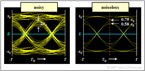
The right graph shows the noisless eye diagram. One can see from this the vertical eye opening in the center of the symbol:

$$\ddot{o}(T_{\rm D} = 0) = 2 \cdot 0.58 \cdot s_0.$$

Together with the noise rms value, we obtain for the worst-case error probability:

$$p_{\rm U} = {\rm Q} \left( \frac{1.16\,{\rm V}/2}{ 0.188\,{\rm V}} \right) \approx {\rm Q}(3.08)\hspace{0.15cm}\underline {\approx 10^{-3}} \hspace{0.05cm}.$$

(5) From the noisless eye diagram, one can see that the signal component at the detection time $T_{\rm D} = 0$ can assume six different values.

In the upper half of the eye, these are:

$$1.)\hspace{0.2cm} g_0 + g_1 + g_{-1} = 0.790\,{\rm V} + 2\cdot 0.105\,{\rm V}= 1\,{\rm V} = s_0$$

$$\Rightarrow \hspace{0.3cm} p_{\rm 1} = {\rm Q} \left( \frac{1\,{\rm V}}{ 0.188\,{\rm V}} \right) \approx 5 \cdot 10^{-8} \hspace{0.05cm},$$

$$2.)\hspace{0.2cm} g_0 = 0.790\,{\rm V} \hspace{0.3cm}\Rightarrow \hspace{0.3cm} p_{\rm 2} = {\rm Q} \left( \frac{0.790\,{\rm V}}{ 0.188\,{\rm V}} \right) \approx 1.3 \cdot 10^{-5} \hspace{0.05cm},$$

$$3.)\hspace{0.2cm} g_0 - g_1 - g_{-1} = 0.580\,{\rm V} = \ddot{o}(T_{\rm D})/2\hspace{0.3cm}\Rightarrow \hspace{0.3cm}p_{\rm 3} = p_{\rm U} \approx 10^{-3} \hspace{0.05cm}.$$

Averaging over these values with appropriate weighting $(p_2$ occurs twice as often as $p_1$ and $p_3)$ gives:

$$p_{\rm S} \ = \ {1}/{4} \cdot (p_{\rm 1} + 2 \cdot p_{\rm 2} + p_{\rm 3}) = {1}/{4} \cdot (5 \cdot 10^{-8} + 2 \cdot 1.3 \cdot 10^{-5} + 10^{-3}) \hspace{0.15cm}\underline { \approx 0.256 \cdot 10^{-3}} \hspace{0.05cm}.$$

Since $p_1$ and $p_2$ are much smaller than $p_3 = p_{\rm U}$, the average error probability is (almost) a factor of $4$ smaller than $p_{\rm U}$.

(6) To reduce the error probability, $s_0$ must be increased. Thus, the approximation $p_{\rm S} ≈ p_{\rm U}/4$ is even more accurate:

$$p_{\rm S} \le 10^{-10}\hspace{0.3cm}\Rightarrow \hspace{0.3cm}p_{\rm U} = {\rm Q} \left( \frac{0.58 \cdot s_0}{ 0.188\,{\rm V}} \right)\le 4 \cdot 10^{-10}\hspace{0.3cm} \Rightarrow \hspace{0.3cm} \frac{0.58 \cdot s_0}{ 0.188\,{\rm V}} \ge 6.15 \hspace{0.3cm}\Rightarrow \hspace{0.3cm}s_0 \ge 1.993\,{\rm V} \hspace{0.15cm}\underline { \approx 2\,{\rm V}} \hspace{0.05cm}.$$