Difference between revisions of "Aufgaben:Exercise 3.1: Cosine-square PDF and PDF with Dirac Functions"
| (24 intermediate revisions by 4 users not shown) | |||
| Line 1: | Line 1: | ||
| − | {{quiz-Header|Buchseite= | + | {{quiz-Header|Buchseite=Theory_of_Stochastic_Signals/Probability_Density_Function |
}} | }} | ||
| − | [[File:P_ID143__Sto_A_3_1.png|right|]] | + | [[File:P_ID143__Sto_A_3_1.png|right|frame|Cosine–square PDF (top), and <br>Dirac delta PDF (bottom)]] |
| − | + | The graph shows the probability density functions $\rm (PDF)$ of two random variables $x$ and $y$. | |
| − | + | *The PDF of the random variable $x$ in analytical form is: | |
| − | :$$f_x(x)=\left\{\begin{array}{*{4}{c}}A | + | :$$f_x(x)=\left\{\begin{array}{*{4}{c}}A \cdot \cos^2({\pi}/{4}\cdot x) &\rm for\hspace{0.1cm} -2\le \it x\le \rm +2, \\0 & \rm else. \\\end{array}\right.$$ |
| − | + | *The PDF of the random variable $y$ consists of a total of five Dirac delta functions with the weights given in the graph. | |
| − | |||
| − | + | If we consider these random variables as instantaneous values of two random signals $x(t)$ and $y(t)$, <br>it is obvious that both signals are "amplitude limited" to the range $\pm 2$. . | |
| − | |||
| − | === | + | |
| + | |||
| + | |||
| + | Hints: | ||
| + | *The exercise belongs to the chapter [[Theory_of_Stochastic_Signals/Probability_Density_Function|Probability Density Function]]. | ||
| + | *Reference is also made to the chapter [[Theory_of_Stochastic_Signals/From_Random_Experiment_to_Random_Variable|From Random Experiment to Random Variable]]. | ||
| + | *The following integral equation holds: | ||
| + | :$$\int \cos^{\rm 2}( ax)\, {\rm d}x=\frac{x}{2}+\frac{1}{4 a}\cdot \sin(2 ax).$$ | ||
| + | |||
| + | |||
| + | ===Questions=== | ||
<quiz display=simple> | <quiz display=simple> | ||
| − | { | + | {Which of the following statements are absolutely true? |
|type="[]"} | |type="[]"} | ||
| − | + | + | + The random variable $x$ is continuous in value. |
| − | + | + | + The random variable $y$ is discrete in value. |
| − | - | + | - The randomness of $y$ is also discrete in time. |
| − | + | + | + The PDF says nothing regarding "discrete-time/continuous-time." |
| − | { | + | {Calculate the parameter $A$ of the PDF $f_x(x)$. |
|type="{}"} | |type="{}"} | ||
| − | $A$ | + | $A \ = \ $ { 0.5 3% } |
| − | { | + | {What is the probability that $x = 0$ holds? |
|type="{}"} | |type="{}"} | ||
| − | $Pr(x\ =\ | + | ${\rm Pr}(x = 0)\ = \ $ { 0. } |
| − | { | + | {What is the probability that $x > 0$ ? |
|type="{}"} | |type="{}"} | ||
| − | $Pr(x | + | ${\rm Pr}(x > 0)\ = \ $ { 0.5 3% } |
| − | { | + | {What is the probability that $y > 0$ ? |
|type="{}"} | |type="{}"} | ||
| − | $Pr(y | + | ${\rm Pr}(y > 0)\ = \ $ { 0.3 3% } |
| − | { | + | {What is the probability that $|\hspace{0.05cm}y\hspace{0.05cm}|$ is smaller than $1$ ? |
|type="{}"} | |type="{}"} | ||
| − | $Pr(|y| | + | ${\rm Pr}(|\hspace{0.05cm}y\hspace{0.05cm}| <1)\ = \ $ { 0.4 3% } |
| − | { | + | {What is the probability that $|\hspace{0.05cm}x\hspace{0.05cm}|$ is smaller than $1$ ? |
|type="{}"} | |type="{}"} | ||
| − | $Pr(|x| | + | ${\rm Pr}(|\hspace{0.05cm}x\hspace{0.05cm}| <1)\ = \ $ { 0.818 3% } |
| − | |||
</quiz> | </quiz> | ||
| − | === | + | ===Solution=== |
{{ML-Kopf}} | {{ML-Kopf}} | ||
| − | + | '''(1)''' Correct are <u>statements 1, 2, and 4</u>: | |
| + | * $x$ is continuous in value. | ||
| + | * $y$ is discrete in value $(M = 5)$. | ||
| + | *The PDF does not provide information about whether a random variable is discrete or continuous in time. | ||
| + | |||
| + | |||
| + | |||
| + | [[File:EN_Sto_A_3_1_b.png|right|frame|For calculating the PDF area]] | ||
| + | '''(2)''' The area under the PDF must yield $1$: | ||
| + | *By simple geometric reasoning, one arrives at the result $\underline{A=0.5}$. | ||
| + | |||
| − | |||
| − | |||
| − | |||
| − | + | '''(3)''' The probability that the continuous-valued random variable $x$ takes a fixed value $x_0$ is always negligibly small: | |
| + | :$$\underline{{\rm Pr}(x = 0) = 0}.$$ | ||
| + | *On the other hand, for the discrete value random variable $y$ holds according to the specification: | ||
| + | :$${\rm Pr}(y = 0) = 0.4,$$ | ||
| + | :because the given weight of the Dirac delta function at $y = 0$ is $0.4$. | ||
| − | |||
| − | |||
| − | |||
| − | + | '''(4)''' Because of ${{\rm Pr}(x = 0) = 0}$ and the PDF symmetry, we get $\underline{{\rm Pr}(x > 0) = 0.5}$. | |
| − | |||
| − | :< | + | |
| − | :$$\rm Pr(|\ | + | |
| + | '''(5)''' Since $y$ is a discrete random variable, the probabilities for $y = 1$ and $y = 2$ add up: | ||
| + | :$${\rm Pr}(y >0) = {\rm Pr}(y = 1) + {\rm Pr}( y = 2) \hspace{0.15cm}\underline {= 0.3}.$$ | ||
| + | |||
| + | |||
| + | |||
| + | '''(6)''' The event $|\hspace{0.05cm} y \hspace{0.05cm} | < 1$ here is identical to $y = 0$. Thus we obtain: | ||
| + | :$${\rm Pr}(|\hspace{0.05cm}y\hspace{0.05cm}| < 1) = {\rm Pr}( y = 0)\hspace{0.15cm}\underline { = 0.4}.$$ | ||
| + | |||
| + | |||
| + | '''(7)''' The probability we are looking for is equal to the integral from $-1$ to $+1$ over the PDF of the continuous random variable $x$. | ||
| + | *Taking into account the symmetry and the given equation, we obtain: | ||
| + | :$${\rm Pr}(|\hspace{0.05cm} x\hspace{0.05cm}|<1)=2 \cdot \int_{0}^{1}{1}/{2}\cdot \cos^2({\pi}/{4}\cdot x)\hspace{0.1cm}{\rm d}x={x}/{2}+{1}/{\pi}\cdot \sin({\pi}/{2}\cdot x)\Big |_{\rm 0}^{\rm 1}=\rm{1}/{2} + {1}/{\pi} | ||
\hspace{0.15cm}\underline{ | \hspace{0.15cm}\underline{ | ||
\approx 0.818}.$$ | \approx 0.818}.$$ | ||
| − | |||
{{ML-Fuß}} | {{ML-Fuß}} | ||
| − | [[Category: | + | [[Category:Theory of Stochastic Signals: Exercises|^3.1 Probability Density Function^]] |
Latest revision as of 17:53, 8 February 2022
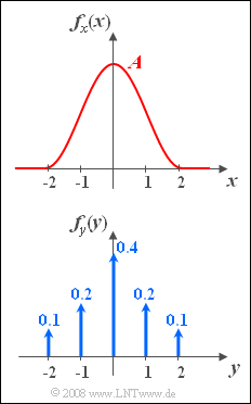
The graph shows the probability density functions $\rm (PDF)$ of two random variables $x$ and $y$.
- The PDF of the random variable $x$ in analytical form is:
- $$f_x(x)=\left\{\begin{array}{*{4}{c}}A \cdot \cos^2({\pi}/{4}\cdot x) &\rm for\hspace{0.1cm} -2\le \it x\le \rm +2, \\0 & \rm else. \\\end{array}\right.$$
- The PDF of the random variable $y$ consists of a total of five Dirac delta functions with the weights given in the graph.
If we consider these random variables as instantaneous values of two random signals $x(t)$ and $y(t)$,
it is obvious that both signals are "amplitude limited" to the range $\pm 2$. .
Hints:
- The exercise belongs to the chapter Probability Density Function.
- Reference is also made to the chapter From Random Experiment to Random Variable.
- The following integral equation holds:
- $$\int \cos^{\rm 2}( ax)\, {\rm d}x=\frac{x}{2}+\frac{1}{4 a}\cdot \sin(2 ax).$$
Questions
Solution
- $x$ is continuous in value.
- $y$ is discrete in value $(M = 5)$.
- The PDF does not provide information about whether a random variable is discrete or continuous in time.
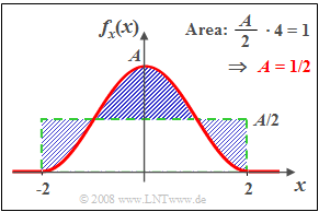
(2) The area under the PDF must yield $1$:
- By simple geometric reasoning, one arrives at the result $\underline{A=0.5}$.
(3) The probability that the continuous-valued random variable $x$ takes a fixed value $x_0$ is always negligibly small:
- $$\underline{{\rm Pr}(x = 0) = 0}.$$
- On the other hand, for the discrete value random variable $y$ holds according to the specification:
- $${\rm Pr}(y = 0) = 0.4,$$
- because the given weight of the Dirac delta function at $y = 0$ is $0.4$.
(4) Because of ${{\rm Pr}(x = 0) = 0}$ and the PDF symmetry, we get $\underline{{\rm Pr}(x > 0) = 0.5}$.
(5) Since $y$ is a discrete random variable, the probabilities for $y = 1$ and $y = 2$ add up:
- $${\rm Pr}(y >0) = {\rm Pr}(y = 1) + {\rm Pr}( y = 2) \hspace{0.15cm}\underline {= 0.3}.$$
(6) The event $|\hspace{0.05cm} y \hspace{0.05cm} | < 1$ here is identical to $y = 0$. Thus we obtain:
- $${\rm Pr}(|\hspace{0.05cm}y\hspace{0.05cm}| < 1) = {\rm Pr}( y = 0)\hspace{0.15cm}\underline { = 0.4}.$$
(7) The probability we are looking for is equal to the integral from $-1$ to $+1$ over the PDF of the continuous random variable $x$.
- Taking into account the symmetry and the given equation, we obtain:
- $${\rm Pr}(|\hspace{0.05cm} x\hspace{0.05cm}|<1)=2 \cdot \int_{0}^{1}{1}/{2}\cdot \cos^2({\pi}/{4}\cdot x)\hspace{0.1cm}{\rm d}x={x}/{2}+{1}/{\pi}\cdot \sin({\pi}/{2}\cdot x)\Big |_{\rm 0}^{\rm 1}=\rm{1}/{2} + {1}/{\pi} \hspace{0.15cm}\underline{ \approx 0.818}.$$

