Difference between revisions of "Aufgaben:Exercise 3.6: Transversal Filter of the Optimal Nyquist Equalizer"
m (Text replacement - "Category:Aufgaben zu Digitalsignalübertragung" to "Category:Digital Signal Transmission: Exercises") |
|||
| (4 intermediate revisions by 2 users not shown) | |||
| Line 1: | Line 1: | ||
| − | {{quiz-Header|Buchseite= | + | {{quiz-Header|Buchseite=Digital_Signal_Transmission/Linear_Nyquist_Equalization |
}} | }} | ||
| − | [[File:P_ID1432__Dig_A_3_6.png|right|frame| | + | [[File:P_ID1432__Dig_A_3_6.png|right|frame|Transversal filter of the <br>Optimal Nyquist Equalizer]] |
| − | + | At the input of the symmetric second order transversal filter $(N = 2)$ shown in the diagram there is a triangular pulse $($normalized to $1)$: | |
:$$g_x(t) = \left\{ \begin{array}{c} 1 - {|\hspace{0.05cm}t\hspace{0.05cm}|}/{(2T)} \\ | :$$g_x(t) = \left\{ \begin{array}{c} 1 - {|\hspace{0.05cm}t\hspace{0.05cm}|}/{(2T)} \\ | ||
\\ 0 \\ \end{array} \right. | \\ 0 \\ \end{array} \right. | ||
| − | \begin{array}{*{1}c} {\rm{ | + | \begin{array}{*{1}c} {\rm{for}}\\ \\ {\rm{for}} \\ \end{array} |
\begin{array}{*{20}c}|\hspace{0.05cm}t\hspace{0.05cm}| \le 2\hspace{0.05cm}T, \\ \\ |\hspace{0.05cm}t\hspace{0.05cm}| \ge 2\hspace{0.05cm}T. \\ | \begin{array}{*{20}c}|\hspace{0.05cm}t\hspace{0.05cm}| \le 2\hspace{0.05cm}T, \\ \\ |\hspace{0.05cm}t\hspace{0.05cm}| \ge 2\hspace{0.05cm}T. \\ | ||
\end{array}$$ | \end{array}$$ | ||
| − | + | If all filter coefficients $k_0$, $k_1$ and $k_2$ are nonzero, then the following holds for the pulse at the output: | |
:$$g_y(t) \ = k_0 \cdot g_x(t) + k_1 \cdot \big[ g_x(t-T)+ | :$$g_y(t) \ = k_0 \cdot g_x(t) + k_1 \cdot \big[ g_x(t-T)+ | ||
g_x(t+T) \big] + k_2 \cdot \big[ g_x(t-2T)+ g_x(t+2T) | g_x(t+T) \big] + k_2 \cdot \big[ g_x(t-2T)+ g_x(t+2T) | ||
\big]\hspace{0.05cm}.$$ | \big]\hspace{0.05cm}.$$ | ||
| − | + | By appropriate choice of filter coefficients $k_0$, $k_1$ and $k_2$, the output pulse can satisfy the following conditions: | |
:$$g_0 = g_y(t = 0) = 1,\hspace{0.2cm}g_1 = g_y(t = \pm T) = | :$$g_0 = g_y(t = 0) = 1,\hspace{0.2cm}g_1 = g_y(t = \pm T) = | ||
0,\hspace{0.2cm}g_2 = g_y(t = \pm 2 T) = 0 \hspace{0.05cm}.$$ | 0,\hspace{0.2cm}g_2 = g_y(t = \pm 2 T) = 0 \hspace{0.05cm}.$$ | ||
| − | * | + | *A first order filter $(N = 1)$ is obtained from the above arrangement and equation by setting the coefficient $k_2 = 0$. |
| − | * | + | |
| − | + | *Then, by appropriate choice of $k_0$ and $k_1$, $g_0 = 1$ and $g_1 = 0$ can be obtained. However, in this case, always will be $g_2 ≠ 0$. | |
| − | |||
| − | + | Note: The exercise belongs to the chapter [[Digital_Signal_Transmission/Linear_Nyquist_Equalization|"Linear Nyquist Equalization"]]. | |
| − | |||
| − | === | + | ===Questions=== |
<quiz display=simple> | <quiz display=simple> | ||
| − | { | + | {What are the optimal coefficients for the first order filter ⇒ $k_2 = 0$? |
|type="{}"} | |type="{}"} | ||
$k_0\ = \ $ { 2 3% } | $k_0\ = \ $ { 2 3% } | ||
$k_1\ = \ $ { -1.03--0.97 } | $k_1\ = \ $ { -1.03--0.97 } | ||
| − | { | + | {What are the output values at time points $t = 2T$ and $t = 3T$? |
|type="{}"} | |type="{}"} | ||
$g_2\ = \ $ { -0.515--0.485 } | $g_2\ = \ $ { -0.515--0.485 } | ||
$g_3\ = \ $ { 0 3% } | $g_3\ = \ $ { 0 3% } | ||
| − | { | + | {What are the optimal coefficients for the second order filter $(N = 2)$? |
|type="{}"} | |type="{}"} | ||
$k_0\ = \ $ { 3 3% } | $k_0\ = \ $ { 3 3% } | ||
| Line 52: | Line 50: | ||
$k_2\ = \ $ { 1 3% } | $k_2\ = \ $ { 1 3% } | ||
| − | { | + | {What are the output values at time points $t = 3T$ and $t = 4T$? |
|type="{}"} | |type="{}"} | ||
$g_3\ = \ $ { 0.5 3% } | $g_3\ = \ $ { 0.5 3% } | ||
| Line 58: | Line 56: | ||
</quiz> | </quiz> | ||
| − | === | + | ===Solution=== |
{{ML-Kopf}} | {{ML-Kopf}} | ||
| − | '''(1)''' | + | '''(1)''' The input pulse $g_x(t)$ is given by the following samples at multiples of $T$: |
:$$g_x(t = 0) = 1,\hspace{0.2cm}g_x(t = \pm T) = | :$$g_x(t = 0) = 1,\hspace{0.2cm}g_x(t = \pm T) = | ||
0.5,\hspace{0.2cm}g_x(t = \pm 2 T) = ... = 0 | 0.5,\hspace{0.2cm}g_x(t = \pm 2 T) = ... = 0 | ||
\hspace{0.05cm}.$$ | \hspace{0.05cm}.$$ | ||
| − | * | + | *Thus, the following system of equations can be set up: |
| + | [[File:P_ID1433__Dig_A_3_6_b.png|right|frame|Output pulse for $N = 1$]] | ||
:$$t = 0\hspace{-0.1cm}:\hspace{0.2cm}g_0 \hspace{-0.1cm} \ = \ \hspace{-0.1cm} k_0 \cdot 1.0 + k_1 \cdot 2 | :$$t = 0\hspace{-0.1cm}:\hspace{0.2cm}g_0 \hspace{-0.1cm} \ = \ \hspace{-0.1cm} k_0 \cdot 1.0 + k_1 \cdot 2 | ||
\cdot 0.5 = 1\hspace{0.05cm},$$ | \cdot 0.5 = 1\hspace{0.05cm},$$ | ||
:$$t = T\hspace{-0.1cm}:\hspace{0.2cm}g_1 \hspace{-0.1cm} \ = \ \hspace{-0.1cm} k_0 \cdot 0.5 + k_1 \cdot 1.0 = 0 | :$$t = T\hspace{-0.1cm}:\hspace{0.2cm}g_1 \hspace{-0.1cm} \ = \ \hspace{-0.1cm} k_0 \cdot 0.5 + k_1 \cdot 1.0 = 0 | ||
\hspace{0.05cm}.$$ | \hspace{0.05cm}.$$ | ||
| − | + | *From these equations, it follows that $k_0 \ \underline {= \ 2}$ and $k_1 \ \underline {= \ –1}$. | |
| − | |||
| − | '''(2)''' | + | '''(2)''' The values $g_0 = 1$ and $g_1 = 0$ have already been used as a basis for the optimization and are therefore undisputed. |
| − | * | + | *At time $t = 2T$, the output results, where $k_{-1} = k_1 = -1$: |
:$$g_2 = g_y(t = 2 T) = g_x(t = T) \cdot k_{-1}\hspace{0.15cm}\underline { = -0.5 = | :$$g_2 = g_y(t = 2 T) = g_x(t = T) \cdot k_{-1}\hspace{0.15cm}\underline { = -0.5 = | ||
g_{-2}} \hspace{0.05cm}.$$ | g_{-2}} \hspace{0.05cm}.$$ | ||
| − | * | + | *Since all input values are zero at times $2T$, $3T$ and $4T$ ⇒ $g_3 = g_y(t = 3T) \underline {= \ 0}$. |
| − | * | + | *This gives the output pulse $g_y(t)$ as shown in the sketch. |
| − | + | '''(3)''' For a second order filter, the system of equations is: | |
| − | '''(3)''' | ||
:$$t = 2T\hspace{-0.1cm}:\hspace{0.2cm}g_2 = k_1 \cdot 0.5 + k_2 \cdot 1.0 = 0 \hspace{0.3cm}\Rightarrow \hspace{0.3cm} k_2 = - 0.5 \cdot k_1\hspace{0.05cm},$$ | :$$t = 2T\hspace{-0.1cm}:\hspace{0.2cm}g_2 = k_1 \cdot 0.5 + k_2 \cdot 1.0 = 0 \hspace{0.3cm}\Rightarrow \hspace{0.3cm} k_2 = - 0.5 \cdot k_1\hspace{0.05cm},$$ | ||
| + | [[File:P_ID1439__Dig_A_3_6_d.png|right|frame|Output pulse for $N = 2$]] | ||
:$$t = T\hspace{-0.1cm}:\hspace{0.2cm}g_1= k_0 \cdot 0.5 +k_1 \cdot 1.0 + k_2 \cdot 0.5 = 0\hspace{0.05cm},$$ | :$$t = T\hspace{-0.1cm}:\hspace{0.2cm}g_1= k_0 \cdot 0.5 +k_1 \cdot 1.0 + k_2 \cdot 0.5 = 0\hspace{0.05cm},$$ | ||
:$$\hspace{1.6cm}\Rightarrow \hspace{0.3cm} | :$$\hspace{1.6cm}\Rightarrow \hspace{0.3cm} | ||
| Line 91: | Line 89: | ||
:$$t = 0\hspace{-0.1cm}:\hspace{0.2cm}g_0 = k_0 \cdot 1.0 + k_1 \cdot 0.5 + k_1 \cdot 0.5 = 1\hspace{0.05cm},$$ | :$$t = 0\hspace{-0.1cm}:\hspace{0.2cm}g_0 = k_0 \cdot 1.0 + k_1 \cdot 0.5 + k_1 \cdot 0.5 = 1\hspace{0.05cm},$$ | ||
:$$\hspace{1.6cm}\Rightarrow \hspace{0.3cm} k_0 = 3 \hspace{0.05cm}.$$ | :$$\hspace{1.6cm}\Rightarrow \hspace{0.3cm} k_0 = 3 \hspace{0.05cm}.$$ | ||
| − | * | + | *Thus, the optimal coefficients are |
:$$k_0 \ \underline {= \ 3},k_1 \ \underline {= \ –2}, k_2 \ \underline {= \ 1}.$$ | :$$k_0 \ \underline {= \ 3},k_1 \ \underline {= \ –2}, k_2 \ \underline {= \ 1}.$$ | ||
| − | '''(4)''' | + | '''(4)''' Proceeding in the same way as in subtask '''(2)''', we obtain $g_4 \ \underline {= \ 0}$ as well as |
:$$g_3 = g_y(t = 3 T) = g_x(t = T) \cdot k_{-2} = 0.5 \cdot 1 | :$$g_3 = g_y(t = 3 T) = g_x(t = T) \cdot k_{-2} = 0.5 \cdot 1 | ||
\hspace{0.15cm}\underline {= 0.5} \hspace{0.05cm}.$$ | \hspace{0.15cm}\underline {= 0.5} \hspace{0.05cm}.$$ | ||
| − | * | + | *However, the two graphs also show that for the triangular shape here, the optimal Nyquist equalization does not improve anything. The eye is "just closed" in all cases: |
| − | |||
:$$N = 0\hspace{-0.1cm}:\hspace{0.2cm} \ddot{o}/2 \hspace{-0.1cm} \ = \ \hspace{-0.1cm} g_0 - 2 \cdot g_1 = 1- 2 \cdot 0.5 = 0 \hspace{0.05cm}, $$ | :$$N = 0\hspace{-0.1cm}:\hspace{0.2cm} \ddot{o}/2 \hspace{-0.1cm} \ = \ \hspace{-0.1cm} g_0 - 2 \cdot g_1 = 1- 2 \cdot 0.5 = 0 \hspace{0.05cm}, $$ | ||
:$$N = 1\hspace{-0.1cm}:\hspace{0.2cm} \ddot{o}/2 \hspace{-0.1cm} \ = \ \hspace{-0.1cm} g_0 - 2 \cdot |g_2 | = 1- 2 \cdot 0.5 = 0 \hspace{0.05cm}, $$ | :$$N = 1\hspace{-0.1cm}:\hspace{0.2cm} \ddot{o}/2 \hspace{-0.1cm} \ = \ \hspace{-0.1cm} g_0 - 2 \cdot |g_2 | = 1- 2 \cdot 0.5 = 0 \hspace{0.05cm}, $$ | ||
| Line 107: | Line 104: | ||
| − | [[Category:Digital Signal Transmission: Exercises|^3.5 | + | [[Category:Digital Signal Transmission: Exercises|^3.5 Linear Nyquist Equalization^]] |
Latest revision as of 16:41, 22 June 2022
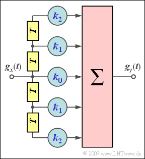
At the input of the symmetric second order transversal filter $(N = 2)$ shown in the diagram there is a triangular pulse $($normalized to $1)$:
- $$g_x(t) = \left\{ \begin{array}{c} 1 - {|\hspace{0.05cm}t\hspace{0.05cm}|}/{(2T)} \\ \\ 0 \\ \end{array} \right. \begin{array}{*{1}c} {\rm{for}}\\ \\ {\rm{for}} \\ \end{array} \begin{array}{*{20}c}|\hspace{0.05cm}t\hspace{0.05cm}| \le 2\hspace{0.05cm}T, \\ \\ |\hspace{0.05cm}t\hspace{0.05cm}| \ge 2\hspace{0.05cm}T. \\ \end{array}$$
If all filter coefficients $k_0$, $k_1$ and $k_2$ are nonzero, then the following holds for the pulse at the output:
- $$g_y(t) \ = k_0 \cdot g_x(t) + k_1 \cdot \big[ g_x(t-T)+ g_x(t+T) \big] + k_2 \cdot \big[ g_x(t-2T)+ g_x(t+2T) \big]\hspace{0.05cm}.$$
By appropriate choice of filter coefficients $k_0$, $k_1$ and $k_2$, the output pulse can satisfy the following conditions:
- $$g_0 = g_y(t = 0) = 1,\hspace{0.2cm}g_1 = g_y(t = \pm T) = 0,\hspace{0.2cm}g_2 = g_y(t = \pm 2 T) = 0 \hspace{0.05cm}.$$
- A first order filter $(N = 1)$ is obtained from the above arrangement and equation by setting the coefficient $k_2 = 0$.
- Then, by appropriate choice of $k_0$ and $k_1$, $g_0 = 1$ and $g_1 = 0$ can be obtained. However, in this case, always will be $g_2 ≠ 0$.
Note: The exercise belongs to the chapter "Linear Nyquist Equalization".
Questions
Solution
- $$g_x(t = 0) = 1,\hspace{0.2cm}g_x(t = \pm T) = 0.5,\hspace{0.2cm}g_x(t = \pm 2 T) = ... = 0 \hspace{0.05cm}.$$
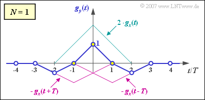
- Thus, the following system of equations can be set up:
- $$t = 0\hspace{-0.1cm}:\hspace{0.2cm}g_0 \hspace{-0.1cm} \ = \ \hspace{-0.1cm} k_0 \cdot 1.0 + k_1 \cdot 2 \cdot 0.5 = 1\hspace{0.05cm},$$
- $$t = T\hspace{-0.1cm}:\hspace{0.2cm}g_1 \hspace{-0.1cm} \ = \ \hspace{-0.1cm} k_0 \cdot 0.5 + k_1 \cdot 1.0 = 0 \hspace{0.05cm}.$$
- From these equations, it follows that $k_0 \ \underline {= \ 2}$ and $k_1 \ \underline {= \ –1}$.
(2) The values $g_0 = 1$ and $g_1 = 0$ have already been used as a basis for the optimization and are therefore undisputed.
- At time $t = 2T$, the output results, where $k_{-1} = k_1 = -1$:
- $$g_2 = g_y(t = 2 T) = g_x(t = T) \cdot k_{-1}\hspace{0.15cm}\underline { = -0.5 = g_{-2}} \hspace{0.05cm}.$$
- Since all input values are zero at times $2T$, $3T$ and $4T$ ⇒ $g_3 = g_y(t = 3T) \underline {= \ 0}$.
- This gives the output pulse $g_y(t)$ as shown in the sketch.
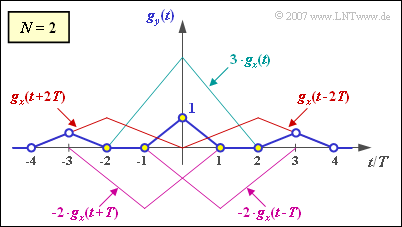
(3) For a second order filter, the system of equations is:
- $$t = 2T\hspace{-0.1cm}:\hspace{0.2cm}g_2 = k_1 \cdot 0.5 + k_2 \cdot 1.0 = 0 \hspace{0.3cm}\Rightarrow \hspace{0.3cm} k_2 = - 0.5 \cdot k_1\hspace{0.05cm},$$
- $$t = T\hspace{-0.1cm}:\hspace{0.2cm}g_1= k_0 \cdot 0.5 +k_1 \cdot 1.0 + k_2 \cdot 0.5 = 0\hspace{0.05cm},$$
- $$\hspace{1.6cm}\Rightarrow \hspace{0.3cm} k_1 = - {2}/{3} \cdot k_0\hspace{0.05cm},$$
- $$t = 0\hspace{-0.1cm}:\hspace{0.2cm}g_0 = k_0 \cdot 1.0 + k_1 \cdot 0.5 + k_1 \cdot 0.5 = 1\hspace{0.05cm},$$
- $$\hspace{1.6cm}\Rightarrow \hspace{0.3cm} k_0 = 3 \hspace{0.05cm}.$$
- Thus, the optimal coefficients are
- $$k_0 \ \underline {= \ 3},k_1 \ \underline {= \ –2}, k_2 \ \underline {= \ 1}.$$
(4) Proceeding in the same way as in subtask (2), we obtain $g_4 \ \underline {= \ 0}$ as well as
- $$g_3 = g_y(t = 3 T) = g_x(t = T) \cdot k_{-2} = 0.5 \cdot 1 \hspace{0.15cm}\underline {= 0.5} \hspace{0.05cm}.$$
- However, the two graphs also show that for the triangular shape here, the optimal Nyquist equalization does not improve anything. The eye is "just closed" in all cases:
- $$N = 0\hspace{-0.1cm}:\hspace{0.2cm} \ddot{o}/2 \hspace{-0.1cm} \ = \ \hspace{-0.1cm} g_0 - 2 \cdot g_1 = 1- 2 \cdot 0.5 = 0 \hspace{0.05cm}, $$
- $$N = 1\hspace{-0.1cm}:\hspace{0.2cm} \ddot{o}/2 \hspace{-0.1cm} \ = \ \hspace{-0.1cm} g_0 - 2 \cdot |g_2 | = 1- 2 \cdot 0.5 = 0 \hspace{0.05cm}, $$
- $$N = 2\hspace{-0.1cm}:\hspace{0.2cm} \ddot{o}/2 \hspace{-0.1cm} \ = \ \hspace{-0.1cm} g_0 - 2 \cdot g_3 = 1- 2 \cdot 0.5 = 0 \hspace{0.05cm}.$$


