Difference between revisions of "Aufgaben:Exercise 3.8: Amplification and Limitation"
From LNTwww
m (Text replacement - "Category:Aufgaben zu Stochastische Signaltheorie" to "Category:Theory of Stochastic Signals: Exercises") |
m (Text replacement - "rms value" to "standard deviation") |
||
| (11 intermediate revisions by 2 users not shown) | |||
| Line 1: | Line 1: | ||
| − | {{quiz-Header|Buchseite= | + | {{quiz-Header|Buchseite=Theory_of_Stochastic_Signals/Exponentially_Distributed_Random_Variables |
}} | }} | ||
| − | [[File:P_ID130__Sto_A_3_8.png|right|frame| | + | [[File:P_ID130__Sto_A_3_8.png|right|frame|Amplification and limitation<br>of the random variable $x$]] |
| − | + | We consider a random signal $x(t)$ with symmetric probability density function $\rm (PDF)$: | |
| − | :$$f_x(x)=A\cdot | + | :$$f_x(x)=A\cdot \rm e^{\rm -2 \hspace{0.05cm}\cdot \hspace{0.05cm}|\it x|}.$$ |
| − | * | + | *This signal is applied to the input of a nonlinearity with the characteristic curve (see lower figure): |
| − | :$$y=\left\{\begin{array}{*{4}{c}}0 &\rm | + | :$$y=\left\{\begin{array}{*{4}{c}}0 &\rm for\hspace{0.2cm} \it x <\rm 0, \\\rm2\it x & \rm for\hspace{0.2cm} \rm 0\le \it x\le \rm 0.5, \\1 & \rm for\hspace{0.2cm}\it x > \rm 0.5\\\end{array}\right.$$ |
| − | * | + | *The characteristic sketched below limits the variable $x(t)$ at the input asymmetrically and amplifies it in the linear range.<br><br> |
| − | |||
| Line 19: | Line 18: | ||
| − | + | Hints: | |
| − | + | *The exercise belongs to the chapter [[Theory_of_Stochastic_Signals/Exponentially_Distributed_Random_Variables|Exponentially Distributed Random Variable]]. | |
| − | + | * Use the HTML5/JavaScript– applet [[Applets:PDF,_CDF_and_Moments_of_Special_Distributions|PDF, CDF and Moments of Special Distributions]] to check your results. | |
| − | * | + | *Given the following definite integral: |
| − | |||
| − | * | ||
:$$\int_{0}^{\infty}\it x^n\cdot\rm e^{-\it a \hspace{0.03cm}\cdot \hspace{0.03cm}x}\, d{\it x} =\frac{\it n{\rm !}}{\it a^{n}}.$$ | :$$\int_{0}^{\infty}\it x^n\cdot\rm e^{-\it a \hspace{0.03cm}\cdot \hspace{0.03cm}x}\, d{\it x} =\frac{\it n{\rm !}}{\it a^{n}}.$$ | ||
| − | === | + | ===Questions=== |
<quiz display=simple> | <quiz display=simple> | ||
| − | { | + | {Calculate the function value $A= f_x(0)$ of the PDF at the location $x = 0$. |
|type="{}"} | |type="{}"} | ||
| − | $A \ = \ $ | + | $A \ = \ $ { 1 3% } |
| − | { | + | {Calculate the moments $m_k$ of the random variable $x$. Reason that all moments with odd index are zero. How big is the standard deviation? |
|type="{}"} | |type="{}"} | ||
$\sigma_x \ = \ $ { 0.707 3% } | $\sigma_x \ = \ $ { 0.707 3% } | ||
| − | { | + | {What is the value of the kurtosis of the random variable $x$? |
|type="{}"} | |type="{}"} | ||
$K_x \ = \ $ { 6 3% } | $K_x \ = \ $ { 6 3% } | ||
| − | { | + | {What is the probability that $x$ exceeds $0.5$ ? |
|type="{}"} | |type="{}"} | ||
${\rm Pr}(x > 0.5) \ = \ $ { 18.4 3% } $\ \%$ | ${\rm Pr}(x > 0.5) \ = \ $ { 18.4 3% } $\ \%$ | ||
| − | { | + | {Which of the following statements are true regarding the PDF $f_y(y)$ ? |
|type="[]"} | |type="[]"} | ||
| − | + | + | + The PDF contains a Dirac delta function at $y = 0$. |
| − | - | + | - The PDF contains a Dirac delta function at $y = 0.5$. |
| − | + | + | + The PDF contains a Dirac delta function at $y = 1$. |
| − | { | + | {What is the continuous part of the PDF $f_y(y)$? What value results for $y = 0.5$ ? |
|type="{}"} | |type="{}"} | ||
$f_y(y = 0.5) \ = \ $ { 0.304 3% } | $f_y(y = 0.5) \ = \ $ { 0.304 3% } | ||
| − | { | + | {What is the mean of the bounded and amplified random variable $y$? |
|type="{}"} | |type="{}"} | ||
$m_y \ = \ $ { 0.316 3% } | $m_y \ = \ $ { 0.316 3% } | ||
| − | |||
</quiz> | </quiz> | ||
| − | === | + | ===Solution=== |
{{ML-Kopf}} | {{ML-Kopf}} | ||
| − | '''(1)''' | + | '''(1)''' The area under the probability density function yields |
:$$\it F=\rm 2\cdot \it A\int_{\rm 0}^{\infty}\hspace{-0.15cm}\rm e^{\rm -2\it x}\, \rm d \it x=\frac{\rm 2\cdot \it A}{\rm -2}\cdot \rm e^{\rm -2\it x}\Big|_{\rm 0}^{\infty}=\it A.$$ | :$$\it F=\rm 2\cdot \it A\int_{\rm 0}^{\infty}\hspace{-0.15cm}\rm e^{\rm -2\it x}\, \rm d \it x=\frac{\rm 2\cdot \it A}{\rm -2}\cdot \rm e^{\rm -2\it x}\Big|_{\rm 0}^{\infty}=\it A.$$ | ||
| − | * | + | *Since this area must be equal by definition $F = 1$ ⇒ $\underline{A = 1}$. |
| − | '''(2)''' | + | '''(2)''' All moments with odd index $k$ are equal to zero due to the symmetrical PDF. |
| − | * | + | *For even $k$ the left part of the PDF can be mirrored into the right one and we get: |
:$$\it m_k=\rm 2 \cdot \int_{\rm 0}^{\infty}\hspace{-0.15cm}\it x^{k}\cdot \rm e^{-\rm 2\it x}\,\rm d \it x=\frac{\rm 2\cdot\rm\Gamma(\it k{\rm +}\rm 1)}{\rm 2^{\it k{\rm +}\rm 1}}=\frac{\it k{\rm !}}{\rm 2^{\it k}}.$$ | :$$\it m_k=\rm 2 \cdot \int_{\rm 0}^{\infty}\hspace{-0.15cm}\it x^{k}\cdot \rm e^{-\rm 2\it x}\,\rm d \it x=\frac{\rm 2\cdot\rm\Gamma(\it k{\rm +}\rm 1)}{\rm 2^{\it k{\rm +}\rm 1}}=\frac{\it k{\rm !}}{\rm 2^{\it k}}.$$ | ||
| − | * | + | *From this it follows with $k = 2$ considering the mean $m_1 = 0$: |
| − | :$$m_{\rm 2}=\frac{\rm 2!}{\rm 2^2}={\rm 0.5\hspace{0.5cm}bzw.\hspace{0 | + | :$$m_{\rm 2}=\frac{\rm 2!}{\rm 2^2}={\rm 0.5\hspace{0.5cm}bzw.\hspace{0.5cm} }\sigma_x=\sqrt{ m_{\rm 2}}\hspace{0.15cm}\underline{=\rm 0.707}.$$ |
| − | [[File:P_ID131__Sto_A_3_8_e.png|right|frame| | + | [[File:P_ID131__Sto_A_3_8_e.png|right|frame|PDF after amplification and boundary]] |
| − | '''(3)''' | + | '''(3)''' The fourth-order central moment is $\mu_4 = m_4 = 4!/2^4 = 1.5$. |
| − | * | + | *From this follows for the kurtosis: |
:$$K_{x}=\frac{ \mu_{\rm 4}}{ \sigma_{\it x}^{4}}=\frac{1.5}{0.25}\hspace{0.15cm}\underline{=\rm 6}.$$ | :$$K_{x}=\frac{ \mu_{\rm 4}}{ \sigma_{\it x}^{4}}=\frac{1.5}{0.25}\hspace{0.15cm}\underline{=\rm 6}.$$ | ||
| − | '''(4)''' | + | '''(4)''' Using the result from '''(1)''' we get: |
:$${\rm Pr}( x> 0.5)=\int_{0.5}^{\infty}{\rm e}^{- 2 x}\,{\rm d}x=\frac{\rm 1}{\rm 2\rm e}\hspace{0.15cm}\underline{=\rm 18.4\%}.$$ | :$${\rm Pr}( x> 0.5)=\int_{0.5}^{\infty}{\rm e}^{- 2 x}\,{\rm d}x=\frac{\rm 1}{\rm 2\rm e}\hspace{0.15cm}\underline{=\rm 18.4\%}.$$ | ||
| − | '''(5)''' | + | '''(5)''' Correct are the <u>solutions 1 and 3</u>: |
| − | * | + | *The PDF $f_y(y)$ involves a Dirac delta function at the point $y= 0$ with weight ${\rm Pr}(x < 0) = 0.5$. |
| − | * | + | *In addition, another Dirac delta function at $y= 1$ with weight ${\rm Pr}(x > 0.5) = 0.184$. |
| − | '''(6)''' | + | '''(6)''' The signal range $0 \le x \le 0.5$ is linearly mapped to the range $0 \le y \le 1$ at the output. |
| − | * | + | *The derivative of the characteristic curve is constantly equal to $2$ (amplification). From this one obtains: |
:$$f_y(y)=\frac{f_x(x)}{|g'(x)|}\Bigg|_{x=h(y)}=\frac{\rm e^{-\rm 2\it x}}{\rm 2}\Bigg|_{\it x={\it y}/{\rm 2}}=0.5 \cdot {\rm e^{\it -y}} .$$ | :$$f_y(y)=\frac{f_x(x)}{|g'(x)|}\Bigg|_{x=h(y)}=\frac{\rm e^{-\rm 2\it x}}{\rm 2}\Bigg|_{\it x={\it y}/{\rm 2}}=0.5 \cdot {\rm e^{\it -y}} .$$ | ||
| − | * | + | *For $y= 0.5$ accordingly, the continuous PDF component is |
:$$f_y(y = 0.5)\hspace{0.15cm}\underline{\approx 0.304}.$$ | :$$f_y(y = 0.5)\hspace{0.15cm}\underline{\approx 0.304}.$$ | ||
| − | '''(7)''' | + | '''(7)''' For the mean value of the random variable $y$ holds: |
:$$m_y=\frac{1}{\rm 2\rm e} \cdot 1 +\int_{\rm 0}^{\rm 1}\frac{\it y}{\rm 2}\cdot \rm e^{\it -y}\, \rm d \it y=\frac{\rm 1}{\rm 2\rm e}{\rm +}\frac{\rm 1}{\rm 2}-\frac{\rm 1}{\rm e}=\frac{\rm 1}{\rm 2}-\frac{\rm 1}{\rm 2 e}\hspace{0.15cm}\underline{=\rm 0.316}.$$ | :$$m_y=\frac{1}{\rm 2\rm e} \cdot 1 +\int_{\rm 0}^{\rm 1}\frac{\it y}{\rm 2}\cdot \rm e^{\it -y}\, \rm d \it y=\frac{\rm 1}{\rm 2\rm e}{\rm +}\frac{\rm 1}{\rm 2}-\frac{\rm 1}{\rm e}=\frac{\rm 1}{\rm 2}-\frac{\rm 1}{\rm 2 e}\hspace{0.15cm}\underline{=\rm 0.316}.$$ | ||
| − | * | + | *The first term is from the Dirac delta at $y= 1$, the second from the continuous PDF component. |
{{ML-Fuß}} | {{ML-Fuß}} | ||
| − | [[Category:Theory of Stochastic Signals: Exercises|^3.6 | + | [[Category:Theory of Stochastic Signals: Exercises|^3.6 Exponentially Distributed Random Variables^]] |
Latest revision as of 13:11, 17 February 2022

Amplification and limitation
of the random variable $x$
of the random variable $x$
We consider a random signal $x(t)$ with symmetric probability density function $\rm (PDF)$:
- $$f_x(x)=A\cdot \rm e^{\rm -2 \hspace{0.05cm}\cdot \hspace{0.05cm}|\it x|}.$$
- This signal is applied to the input of a nonlinearity with the characteristic curve (see lower figure):
- $$y=\left\{\begin{array}{*{4}{c}}0 &\rm for\hspace{0.2cm} \it x <\rm 0, \\\rm2\it x & \rm for\hspace{0.2cm} \rm 0\le \it x\le \rm 0.5, \\1 & \rm for\hspace{0.2cm}\it x > \rm 0.5\\\end{array}\right.$$
- The characteristic sketched below limits the variable $x(t)$ at the input asymmetrically and amplifies it in the linear range.
Hints:
- The exercise belongs to the chapter Exponentially Distributed Random Variable.
- Use the HTML5/JavaScript– applet PDF, CDF and Moments of Special Distributions to check your results.
- Given the following definite integral:
- $$\int_{0}^{\infty}\it x^n\cdot\rm e^{-\it a \hspace{0.03cm}\cdot \hspace{0.03cm}x}\, d{\it x} =\frac{\it n{\rm !}}{\it a^{n}}.$$
Questions
Solution
(1) The area under the probability density function yields
- $$\it F=\rm 2\cdot \it A\int_{\rm 0}^{\infty}\hspace{-0.15cm}\rm e^{\rm -2\it x}\, \rm d \it x=\frac{\rm 2\cdot \it A}{\rm -2}\cdot \rm e^{\rm -2\it x}\Big|_{\rm 0}^{\infty}=\it A.$$
- Since this area must be equal by definition $F = 1$ ⇒ $\underline{A = 1}$.
(2) All moments with odd index $k$ are equal to zero due to the symmetrical PDF.
- For even $k$ the left part of the PDF can be mirrored into the right one and we get:
- $$\it m_k=\rm 2 \cdot \int_{\rm 0}^{\infty}\hspace{-0.15cm}\it x^{k}\cdot \rm e^{-\rm 2\it x}\,\rm d \it x=\frac{\rm 2\cdot\rm\Gamma(\it k{\rm +}\rm 1)}{\rm 2^{\it k{\rm +}\rm 1}}=\frac{\it k{\rm !}}{\rm 2^{\it k}}.$$
- From this it follows with $k = 2$ considering the mean $m_1 = 0$:
- $$m_{\rm 2}=\frac{\rm 2!}{\rm 2^2}={\rm 0.5\hspace{0.5cm}bzw.\hspace{0.5cm} }\sigma_x=\sqrt{ m_{\rm 2}}\hspace{0.15cm}\underline{=\rm 0.707}.$$

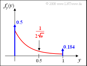
PDF after amplification and boundary
(3) The fourth-order central moment is $\mu_4 = m_4 = 4!/2^4 = 1.5$.
- From this follows for the kurtosis:
- $$K_{x}=\frac{ \mu_{\rm 4}}{ \sigma_{\it x}^{4}}=\frac{1.5}{0.25}\hspace{0.15cm}\underline{=\rm 6}.$$
(4) Using the result from (1) we get:
- $${\rm Pr}( x> 0.5)=\int_{0.5}^{\infty}{\rm e}^{- 2 x}\,{\rm d}x=\frac{\rm 1}{\rm 2\rm e}\hspace{0.15cm}\underline{=\rm 18.4\%}.$$
(5) Correct are the solutions 1 and 3:
- The PDF $f_y(y)$ involves a Dirac delta function at the point $y= 0$ with weight ${\rm Pr}(x < 0) = 0.5$.
- In addition, another Dirac delta function at $y= 1$ with weight ${\rm Pr}(x > 0.5) = 0.184$.
(6) The signal range $0 \le x \le 0.5$ is linearly mapped to the range $0 \le y \le 1$ at the output.
- The derivative of the characteristic curve is constantly equal to $2$ (amplification). From this one obtains:
- $$f_y(y)=\frac{f_x(x)}{|g'(x)|}\Bigg|_{x=h(y)}=\frac{\rm e^{-\rm 2\it x}}{\rm 2}\Bigg|_{\it x={\it y}/{\rm 2}}=0.5 \cdot {\rm e^{\it -y}} .$$
- For $y= 0.5$ accordingly, the continuous PDF component is
- $$f_y(y = 0.5)\hspace{0.15cm}\underline{\approx 0.304}.$$
(7) For the mean value of the random variable $y$ holds:
- $$m_y=\frac{1}{\rm 2\rm e} \cdot 1 +\int_{\rm 0}^{\rm 1}\frac{\it y}{\rm 2}\cdot \rm e^{\it -y}\, \rm d \it y=\frac{\rm 1}{\rm 2\rm e}{\rm +}\frac{\rm 1}{\rm 2}-\frac{\rm 1}{\rm e}=\frac{\rm 1}{\rm 2}-\frac{\rm 1}{\rm 2 e}\hspace{0.15cm}\underline{=\rm 0.316}.$$
- The first term is from the Dirac delta at $y= 1$, the second from the continuous PDF component.