Difference between revisions of "Aufgaben:Exercise 4.4: Two-dimensional Gaussian PDF"
From LNTwww
m (Text replacement - "„" to """) |
|||
| (11 intermediate revisions by 2 users not shown) | |||
| Line 1: | Line 1: | ||
| − | {{quiz-Header|Buchseite= | + | {{quiz-Header|Buchseite=Theory_of_Stochastic_Signals/Two-Dimensional_Gaussian_Random_Variables |
}} | }} | ||
| − | [[File:P_ID261__Sto_A_4_4_neu.png|right|frame| | + | [[File:P_ID261__Sto_A_4_4_neu.png|right|frame|Table: Gaussian error functions]] |
| − | + | We consider two-dimensional random variables, where both components are always assumed to be mean-free. | |
| − | * | + | *The »two-dimensional probability density function« of the random variable $(u, v)$ is: |
:$$f_{uv}(u, v)={1}/{\pi} \cdot {\rm e}^{-(2u^{\rm 2} \hspace{0.05cm}+ \hspace{0.05cm}v^{\rm 2}\hspace{-0.05cm}/\rm 2)}.$$ | :$$f_{uv}(u, v)={1}/{\pi} \cdot {\rm e}^{-(2u^{\rm 2} \hspace{0.05cm}+ \hspace{0.05cm}v^{\rm 2}\hspace{-0.05cm}/\rm 2)}.$$ | ||
| − | * | + | *For another Gaussian two-dimensional random variable $(x, y)$ the following parameters are known: |
:$$\sigma_x= 0.5, \hspace{0.5cm}\sigma_y = 1,\hspace{0.5cm}\rho_{xy} = 1. $$ | :$$\sigma_x= 0.5, \hspace{0.5cm}\sigma_y = 1,\hspace{0.5cm}\rho_{xy} = 1. $$ | ||
| + | *In the adjacent table can be found | ||
| + | #the values of the »Gaussian cumulative distribution function« ${\rm \phi}(x)$ and | ||
| + | #the »complementary function« ${\rm Q}(x) = 1- {\rm \phi}(x)$. | ||
| − | |||
| + | Hints: | ||
| + | *The exercise belongs to the chapter [[Theory_of_Stochastic_Signals/Two-Dimensional_Gaussian_Random_Variables|»Two-dimensional Gaussian Random Variables«]]. | ||
| − | + | *Reference is also made to the chapter [[Theory_of_Stochastic_Signals/Gaussian_Distributed_Random_Variables|»Gaussian distributed random variables«]]. | |
| − | |||
| − | |||
| − | |||
| − | * | ||
| − | |||
| − | |||
| − | |||
| − | |||
| − | |||
| − | === | + | ===Questions=== |
<quiz display=simple> | <quiz display=simple> | ||
| − | { | + | {Which of the statements are true with respect to the two-dimensional random variable $(u, v)$ ? |
|type="[]"} | |type="[]"} | ||
| − | + | + | + The random variables $u$ and $v$ are uncorrelated. |
| − | + | + | + The random variables $u$ and $v$ are statistically independent. |
| − | { | + | {Calculate the two standard deviations $\sigma_u$ and $\sigma_v$. Enter the quotient of the two standard deviations as a check. |
|type="{}"} | |type="{}"} | ||
$\sigma_u/\sigma_v \ = \ $ { 0.5 3% } | $\sigma_u/\sigma_v \ = \ $ { 0.5 3% } | ||
| − | { | + | {Calculate the probability that $u$ is less than $1$. |
|type="{}"} | |type="{}"} | ||
| − | ${\rm Pr}(u < 1)\ = | + | ${\rm Pr}(u < 1)\ = \ $ { 0.9772 3% } |
| − | { | + | {Calculate the probability that the random variable $u$ is less than $1$ and at the same time the random variable $v$ is greater than $1$. |
|type="{}"} | |type="{}"} | ||
| − | ${\rm Pr}\big[(u < 1) ∩ (υ > 1)\big]\ = | + | ${\rm Pr}\big[(u < 1) ∩ (υ > 1)\big]\ = \ $ { 0.1551 3% } |
| − | { | + | {Which of the statements are true for the two-dimensional random variable $(x, y)$? |
|type="[]"} | |type="[]"} | ||
| − | + | + | + The joint probability density function $f_{xy}(x, y)$ is always zero outside the straight line $y = 2x$. |
| − | - | + | - For all pairs of values on the straight line $y = 2x$ holds: $f_{xy}(x, y)= 0.5$. |
| − | + | + | + With respect to the edge PDFs: $f_{x}(x) = f_{u}(u)$ and $f_{y}(y) = f_{v}(v)$ holds. |
| − | { | + | {Calculate the probability that $x$ is less than $1$. |
|type="{}"} | |type="{}"} | ||
| − | ${\rm Pr}(x < 1)\ = | + | ${\rm Pr}(x < 1)\ = \ $ { 0.9772 3% } |
| − | { | + | {Now calculate the probability that the random variable $x$ is less than $1$ and at the same time the random variable $y$ is greater than $1$. |
|type="{}"} | |type="{}"} | ||
| − | ${\rm Pr}\big[(x < 1) ∩ (y > 1)\big]\ = \ $ | + | ${\rm Pr}\big[(x < 1) ∩ (y > 1)\big]\ = \ $ { 0.1359 3% } |
| Line 75: | Line 70: | ||
</quiz> | </quiz> | ||
| − | === | + | ===Solution=== |
{{ML-Kopf}} | {{ML-Kopf}} | ||
| − | '''(1)''' <u> | + | '''(1)''' <u>Both statements are true</u>: |
| − | * | + | *Comparing the given 2D–PDF with the general 2D–PDF |
:$$f_{uv}(u,v) = \frac{\rm 1}{{\rm 2}\it\pi \cdot \sigma_u \cdot \sigma_v \cdot \sqrt{{\rm 1}-\it \rho_{\it uv}^{\rm 2}}} \cdot \rm exp\left[\frac{\rm 1}{2\cdot (\rm 1-\it \rho_{uv}^{\rm 2}{\rm )}}(\frac{\it u^{\rm 2}}{\it\sigma_u^{\rm 2}} + \frac{\it v^{\rm 2}}{\it\sigma_v^{\rm 2}} - \rm 2\it\rho_{uv}\frac{\it u\cdot \it v}{\sigma_u\cdot \sigma_v}\rm )\right],$$ | :$$f_{uv}(u,v) = \frac{\rm 1}{{\rm 2}\it\pi \cdot \sigma_u \cdot \sigma_v \cdot \sqrt{{\rm 1}-\it \rho_{\it uv}^{\rm 2}}} \cdot \rm exp\left[\frac{\rm 1}{2\cdot (\rm 1-\it \rho_{uv}^{\rm 2}{\rm )}}(\frac{\it u^{\rm 2}}{\it\sigma_u^{\rm 2}} + \frac{\it v^{\rm 2}}{\it\sigma_v^{\rm 2}} - \rm 2\it\rho_{uv}\frac{\it u\cdot \it v}{\sigma_u\cdot \sigma_v}\rm )\right],$$ | ||
| − | :so | + | :so it can be seen that no term with $u \cdot v$ occurs in the exponent, which is only possible with $\rho_{uv} = 0$. |
| − | * | + | *But this means that $u$ and $v$ are uncorrelated. |
| − | * | + | *For Gaussian random variables, however, statistical independence always follows from uncorrelatedness. |
| − | '''(2)''' | + | '''(2)''' With statistical independence holds: |
| − | :$$f_{uv}(u, v) = f_u(u)\cdot f_v(v) | + | :$$f_{uv}(u, v) = f_u(u)\cdot f_v(v) $$ |
| − | f_u(u)=\frac{{\rm e}^{-{\it u^{\rm 2}}/{(2\sigma_u^{\rm 2})}}}{\sqrt{\rm 2\pi}\cdot\sigma_u} , | + | :$$f_u(u)=\frac{{\rm e}^{-{\it u^{\rm 2}}/{(2\sigma_u^{\rm 2})}}}{\sqrt{\rm 2\pi}\cdot\sigma_u} , $$ |
| + | :$$\it f_v{\rm (}v{\rm )}=\frac{{\rm e}^{-{\it v^{\rm 2}}/{{\rm (}{\rm 2}\sigma_v^{\rm 2}{\rm )}}}}{\sqrt{\rm 2\pi}\cdot\sigma_v}.$$ | ||
| − | * | + | *By comparing coefficients, we get $\sigma_u = 0.5$ and $\sigma_v = 1$. |
| − | * | + | *The quotient is thus $\sigma_u/\sigma_v\hspace{0.15cm}\underline{=0.5}$. |
| − | + | '''(3)''' Because $u$ is a continuous random variable: | |
| − | '''(3)''' | ||
:$$\rm Pr(\it u < \rm 1) = \rm Pr(\it u \le \rm 1) =\it F_u\rm (1). $$ | :$$\rm Pr(\it u < \rm 1) = \rm Pr(\it u \le \rm 1) =\it F_u\rm (1). $$ | ||
| − | * | + | *With the mean $m_u = 0$ and the standard deviation $\sigma_u = 0.5$ we get: |
:$$\rm Pr(\it u < \rm 1) = \rm \phi({\rm 1}/{\it\sigma_u})= \rm \phi(\rm 2) \hspace{0.15cm}\underline{=\rm 0.9772}. $$ | :$$\rm Pr(\it u < \rm 1) = \rm \phi({\rm 1}/{\it\sigma_u})= \rm \phi(\rm 2) \hspace{0.15cm}\underline{=\rm 0.9772}. $$ | ||
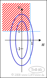
| − | + | [[File:P_ID265__Sto_A_4_4_d.png|right|frame|$\rm Pr\big[(\it u < \rm 1) \cap (\it v > \rm 1)\big]$]] | |
| − | '''(4)''' | + | '''(4)''' Due to the statistical independence between $u$ and $v$ holds: |
:$$\rm Pr\big[(\it u < \rm 1) \cap (\it v > \rm 1)\big] = \rm Pr(\it u < \rm 1)\cdot \rm Pr(\it v > \rm 1).$$ | :$$\rm Pr\big[(\it u < \rm 1) \cap (\it v > \rm 1)\big] = \rm Pr(\it u < \rm 1)\cdot \rm Pr(\it v > \rm 1).$$ | ||
| − | * | + | *The probability ${\rm Pr}(u < 1) =0.9772$ has already been calculated. |
| − | * | + | *For the second probability ${\rm Pr}(v > 1)$ holds for reasons of symmetry: |
:$$\rm Pr(\it v > \rm 1) = \rm Pr(\it v \le \rm (-1) = \it F_v\rm (-1) = \rm \phi(\frac{\rm -1}{\it\sigma_v}) = \rm Q(1) =0.1587$$ | :$$\rm Pr(\it v > \rm 1) = \rm Pr(\it v \le \rm (-1) = \it F_v\rm (-1) = \rm \phi(\frac{\rm -1}{\it\sigma_v}) = \rm Q(1) =0.1587$$ | ||
:$$\Rightarrow \hspace{0.3cm} \rm Pr\big[(\it u < \rm 1) \cap (\it v > \rm 1)\big] = \rm 0.9772\cdot \rm 0.1587 \hspace{0.15cm}\underline{ = \rm 0.1551}.$$ | :$$\Rightarrow \hspace{0.3cm} \rm Pr\big[(\it u < \rm 1) \cap (\it v > \rm 1)\big] = \rm 0.9772\cdot \rm 0.1587 \hspace{0.15cm}\underline{ = \rm 0.1551}.$$ | ||
| − | + | The sketch on the right illustrates the given constellation: | |
| − | * | + | *The PDF contour lines (blue) are stretched ellipses due to $\sigma_v > \sigma_u$ in vertical direction. |
| − | * | + | *Drawn in red (shading) is the area whose probability should be calculated in this subtask. |
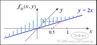
| − | [[File:P_ID266__Sto_A_4_4_e.png|right|frame| | + | [[File:P_ID266__Sto_A_4_4_e.png|right|frame|"Dirac wall" on the correlation line]] |
| − | '''(5)''' | + | '''(5)''' Correct are <u>the first and the third suggested solutions</u>: |
| − | * | + | *Because $\rho_{xy} = 1$ there is a deterministic correlation between $x$ and $y$ |
| − | :⇒ | + | :⇒ All values lie on the straight line $y =K \cdot x$. |
| − | * | + | *Because of the standard deviations $\sigma_x = 0.5$ and $\sigma_y = 1$ it holds $K = 2$. |
| − | * | + | *On this straight line $y = 2x$ ⇒ all PDF values are infinitely large. |
| − | + | *This means: The joint PDF is here a "Dirac wall". | |
| − | * | + | *As you can see from the sketch, the PDF values are Gaussian distributed on the straight line $y = 2x$. |
| − | * | + | *The two marginal probability densities are also Gaussian functions, each with zero mean. |
| − | * | + | *Because of $\sigma_x = \sigma_u$ and $\sigma_y = \sigma_v$ also holds: |
| − | * | + | :$$f_x(x) = f_u(u), \hspace{0.5cm}f_y(y) = f_v(v).$$ |
| − | :$$f_x(x) = f_u(u), | ||
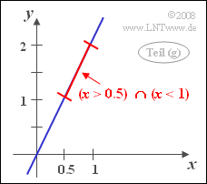
| − | [[File:P_ID274__Sto_A_4_4_g.png|right|frame| | + | [[File:P_ID274__Sto_A_4_4_g.png|right|frame|Probability calculation for the Dirac wall]] |
| − | '''(6)''' | + | '''(6)''' Since the PDF of the random variable $x$ is identical to the PDF $f_u(u)$, it also results in exactly the same probability as calculated in the subtask '''(3)''': |
:$$\rm Pr(\it x < \rm 1) \hspace{0.15cm}\underline{ = \rm 0.9772}.$$ | :$$\rm Pr(\it x < \rm 1) \hspace{0.15cm}\underline{ = \rm 0.9772}.$$ | ||
| − | '''(7)''' | + | '''(7)''' The random event $y > 1$ is identical to the event $x > 0.5$. |
| − | * | + | *Thus, the wanted probability is equal to: |
| − | :$$\rm Pr \big[(\it x | + | :$${\rm Pr}\big[(x < 1) ∩ (y > 1)\big] = \rm Pr \big[ (\it x < \rm 1)\cap (\it x > \rm 0.5) \big] = \it F_x \rm( 1) - \it F_x\rm (0.5). $$ |
| − | * | + | *With the standard deviation $\sigma_x = 0.5$ it follows further: |
:$$\rm Pr \big[(\it x > \rm 0.5) \cap (\it x < \rm 1)\big] = \rm \phi(\rm 2) - \phi(1)=\rm 0.9772- \rm 0.8413\hspace{0.15cm}\underline{=\rm 0.1359}.$$ | :$$\rm Pr \big[(\it x > \rm 0.5) \cap (\it x < \rm 1)\big] = \rm \phi(\rm 2) - \phi(1)=\rm 0.9772- \rm 0.8413\hspace{0.15cm}\underline{=\rm 0.1359}.$$ | ||
| − | |||
{{ML-Fuß}} | {{ML-Fuß}} | ||
| − | [[Category:Theory of Stochastic Signals: Exercises|^4.2 | + | [[Category:Theory of Stochastic Signals: Exercises|^4.2 Gaussian 2D Random Variables^]] |
Latest revision as of 18:37, 9 January 2024

Table: Gaussian error functions
We consider two-dimensional random variables, where both components are always assumed to be mean-free.
- The »two-dimensional probability density function« of the random variable $(u, v)$ is:
- $$f_{uv}(u, v)={1}/{\pi} \cdot {\rm e}^{-(2u^{\rm 2} \hspace{0.05cm}+ \hspace{0.05cm}v^{\rm 2}\hspace{-0.05cm}/\rm 2)}.$$
- For another Gaussian two-dimensional random variable $(x, y)$ the following parameters are known:
- $$\sigma_x= 0.5, \hspace{0.5cm}\sigma_y = 1,\hspace{0.5cm}\rho_{xy} = 1. $$
- In the adjacent table can be found
- the values of the »Gaussian cumulative distribution function« ${\rm \phi}(x)$ and
- the »complementary function« ${\rm Q}(x) = 1- {\rm \phi}(x)$.
Hints:
- The exercise belongs to the chapter »Two-dimensional Gaussian Random Variables«.
- Reference is also made to the chapter »Gaussian distributed random variables«.
Questions
Solution
(1) Both statements are true:
- Comparing the given 2D–PDF with the general 2D–PDF
- $$f_{uv}(u,v) = \frac{\rm 1}{{\rm 2}\it\pi \cdot \sigma_u \cdot \sigma_v \cdot \sqrt{{\rm 1}-\it \rho_{\it uv}^{\rm 2}}} \cdot \rm exp\left[\frac{\rm 1}{2\cdot (\rm 1-\it \rho_{uv}^{\rm 2}{\rm )}}(\frac{\it u^{\rm 2}}{\it\sigma_u^{\rm 2}} + \frac{\it v^{\rm 2}}{\it\sigma_v^{\rm 2}} - \rm 2\it\rho_{uv}\frac{\it u\cdot \it v}{\sigma_u\cdot \sigma_v}\rm )\right],$$
- so it can be seen that no term with $u \cdot v$ occurs in the exponent, which is only possible with $\rho_{uv} = 0$.
- But this means that $u$ and $v$ are uncorrelated.
- For Gaussian random variables, however, statistical independence always follows from uncorrelatedness.
(2) With statistical independence holds:
- $$f_{uv}(u, v) = f_u(u)\cdot f_v(v) $$
- $$f_u(u)=\frac{{\rm e}^{-{\it u^{\rm 2}}/{(2\sigma_u^{\rm 2})}}}{\sqrt{\rm 2\pi}\cdot\sigma_u} , $$
- $$\it f_v{\rm (}v{\rm )}=\frac{{\rm e}^{-{\it v^{\rm 2}}/{{\rm (}{\rm 2}\sigma_v^{\rm 2}{\rm )}}}}{\sqrt{\rm 2\pi}\cdot\sigma_v}.$$
- By comparing coefficients, we get $\sigma_u = 0.5$ and $\sigma_v = 1$.
- The quotient is thus $\sigma_u/\sigma_v\hspace{0.15cm}\underline{=0.5}$.
(3) Because $u$ is a continuous random variable:
- $$\rm Pr(\it u < \rm 1) = \rm Pr(\it u \le \rm 1) =\it F_u\rm (1). $$
- With the mean $m_u = 0$ and the standard deviation $\sigma_u = 0.5$ we get:
- $$\rm Pr(\it u < \rm 1) = \rm \phi({\rm 1}/{\it\sigma_u})= \rm \phi(\rm 2) \hspace{0.15cm}\underline{=\rm 0.9772}. $$

$\rm Pr\big[(\it u < \rm 1) \cap (\it v > \rm 1)\big]$
(4) Due to the statistical independence between $u$ and $v$ holds:
- $$\rm Pr\big[(\it u < \rm 1) \cap (\it v > \rm 1)\big] = \rm Pr(\it u < \rm 1)\cdot \rm Pr(\it v > \rm 1).$$
- The probability ${\rm Pr}(u < 1) =0.9772$ has already been calculated.
- For the second probability ${\rm Pr}(v > 1)$ holds for reasons of symmetry:
- $$\rm Pr(\it v > \rm 1) = \rm Pr(\it v \le \rm (-1) = \it F_v\rm (-1) = \rm \phi(\frac{\rm -1}{\it\sigma_v}) = \rm Q(1) =0.1587$$
- $$\Rightarrow \hspace{0.3cm} \rm Pr\big[(\it u < \rm 1) \cap (\it v > \rm 1)\big] = \rm 0.9772\cdot \rm 0.1587 \hspace{0.15cm}\underline{ = \rm 0.1551}.$$
The sketch on the right illustrates the given constellation:
- The PDF contour lines (blue) are stretched ellipses due to $\sigma_v > \sigma_u$ in vertical direction.
- Drawn in red (shading) is the area whose probability should be calculated in this subtask.

"Dirac wall" on the correlation line
(5) Correct are the first and the third suggested solutions:
- Because $\rho_{xy} = 1$ there is a deterministic correlation between $x$ and $y$
- ⇒ All values lie on the straight line $y =K \cdot x$.
- Because of the standard deviations $\sigma_x = 0.5$ and $\sigma_y = 1$ it holds $K = 2$.
- On this straight line $y = 2x$ ⇒ all PDF values are infinitely large.
- This means: The joint PDF is here a "Dirac wall".
- As you can see from the sketch, the PDF values are Gaussian distributed on the straight line $y = 2x$.
- The two marginal probability densities are also Gaussian functions, each with zero mean.
- Because of $\sigma_x = \sigma_u$ and $\sigma_y = \sigma_v$ also holds:
- $$f_x(x) = f_u(u), \hspace{0.5cm}f_y(y) = f_v(v).$$

Probability calculation for the Dirac wall
(6) Since the PDF of the random variable $x$ is identical to the PDF $f_u(u)$, it also results in exactly the same probability as calculated in the subtask (3):
- $$\rm Pr(\it x < \rm 1) \hspace{0.15cm}\underline{ = \rm 0.9772}.$$
(7) The random event $y > 1$ is identical to the event $x > 0.5$.
- Thus, the wanted probability is equal to:
- $${\rm Pr}\big[(x < 1) ∩ (y > 1)\big] = \rm Pr \big[ (\it x < \rm 1)\cap (\it x > \rm 0.5) \big] = \it F_x \rm( 1) - \it F_x\rm (0.5). $$
- With the standard deviation $\sigma_x = 0.5$ it follows further:
- $$\rm Pr \big[(\it x > \rm 0.5) \cap (\it x < \rm 1)\big] = \rm \phi(\rm 2) - \phi(1)=\rm 0.9772- \rm 0.8413\hspace{0.15cm}\underline{=\rm 0.1359}.$$