Exercise 2.2Z: Discrete Random Variables

Different rectangular signals

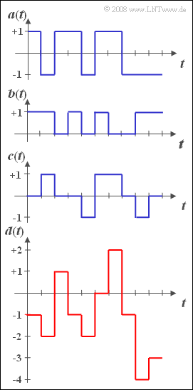
Let be given three discrete random variables $a$, $b$ and $c$, which are defined as the current values of the represented signals. These have the following properties:

The random variable $a$ can take the values $+1$ and $-1$ with equal probability.
The random variable $b$ is also two-point distributed, but with ${\rm Pr}(b = 1) = p$ and ${\rm Pr}(b = 0) = 1 - p$.
The probabilities of $c$ be ${\rm Pr}(c = 0) = 1/2$ and ${\rm Pr}(c = +1) = Pr(c = -1) =1/4$.
There are no statistical dependencies between the three random variables $a$, $b$ and $c$ .
Another random variable $d=a$, $b$ and $c$ is formed from the random variables $d=a-2 b+c$ .

The graph shows sections of these four random variables. It can be seen that $d$ can take all integer values between $-4$ and $+2$ .

Hints:

The exercise belongs to the chapter Moments of a Discrete Random Variable.

The topic of this chapter is illustrated with examples in the (German language) learning video
Momentenberechnung bei diskreten Zufallsgrößen $\Rightarrow$ Calculating Moments for Discrete-Valued Random Variables

Questions

$\sigma_a \ = \ $

$\sigma_b \ = \ $

$\sigma_c \ = \ $

$m_d\ = \ $

$m_{2d}\ = \ $

$\sigma_d\ = \ $

Solution

(1) Due to the symmetry holds:

$$\rm \it m_{\it a}=\rm 0; \hspace{0.5cm}\it m_{\rm 2\it a}=\rm 0.5\cdot (-1)^2 + 0.5\cdot (1)^2{ = 1}.$$

From this one obtains with Steiner's theorem:

$$\it\sigma_a^{\rm 2} = \rm\sqrt{1-0^2}=1 \hspace{0.5cm}or \hspace{0.5cm}\it\sigma_a\hspace{0.15cm} \underline{=\rm 1}.$$

(2) In general, for the $k$–th order moment:

$$ m_{k}=(1-p)\cdot 0^{ k} + p\cdot 1^{k}= p.$$

From this follows with $p = 1/4$:

$$m_{b}= m_{2b}= p, \hspace{0.5cm} \sigma_{\it b}=\sqrt{p\cdot (1- p)}\hspace{0.15cm} \underline{=\rm 0.433} .$$

(3) For the random variable $c$ holds:

$$m_{\it c} = 0\hspace{0.3cm} ({\rm symmetric\hspace{0.1cm}um\hspace{0.1cm}0)},$$

$$ m_{2\it c}= {1}/{4}\cdot(-1)^2+{1}/{2}\cdot 0^2+{1}/{4}\cdot (1)^2={1}/{2} \hspace{0.5cm}$$

$$\Rightarrow \hspace{0.5cm}\sigma_{\it c}=\rm \sqrt{1/2}\hspace{0.15cm} \underline{=0.707}.$$

(4) According to the general rules for expected values, with $p = 0.25$:

$$m_{\it d} = {\rm E}\big[a-2 b+c\big]= {\rm E}\big[a\big] \hspace{0.1cm} -\hspace{0.1cm}\rm 2 \hspace{0.05cm}\cdot\hspace{0.05cm} {\rm E}\big[ b\big]\hspace{0.1cm}+\hspace{0.1cm} {\rm E}\big[ c\big] = m_{ a}\hspace{0.1cm}-\hspace{0.1cm}2\hspace{0.05cm}\cdot\hspace{0.05cm} m_{\it b}\hspace{0.1cm}+\hspace{0.1cm} m_{\it c} = 0-2\hspace{0.05cm}\cdot\hspace{0.05cm} p + 0 \hspace{0.15cm} \underline{= -0.5}.$$

(5) Analogous to the subtask (4) we obtain for the root mean square:

$$m_{2d}= {\rm E}\big[( a-2b+c)^{\rm 2}\big] = {\rm E}\big[a^{\rm 2}\big]\hspace{0.1cm}+\hspace{0.1cm}4\hspace{0.05cm}\cdot\hspace{0.05cm} {\rm E}\big[ b^{\rm 2}\big]\hspace{0.1cm}+\hspace{0.1cm} {\rm E}\big[c^{\rm 2}\big]\hspace{0.1cm} - \hspace{0.1cm}4\hspace{0.05cm}\cdot\hspace{0.05cm} {\rm E}\big[a\hspace{0.05cm}\cdot \hspace{0.05cm}b\big]\hspace{0.1cm}+\hspace{0.1cm} 2\hspace{0.05cm}\cdot\hspace{0.05cm}{\rm E}\big[ a\hspace{0.05cm}\cdot \hspace{0.05cm}c\big]\hspace{0.1cm}-\hspace{0.1cm} 4\hspace{0.05cm}\cdot\hspace{0.05cm}{\rm E}\big[ b\hspace{0.05cm}\cdot \hspace{0.05cm}c\big].$$

But since $a$ and $b$ are statistically independent of each other, also holds:

$${\rm E}\big[a\cdot b\big] = {\rm E}\big[ a\big] \cdot {\rm E}\big[ b\big]= m_{ a}\cdot m_{ b} = 0, \hspace{0.2cm} {\rm da}\hspace{0.2cm} m_{ a}=\rm 0.$$

The same holds for the other mixed terms. Therefore, using $p = 0.25$, we obtain:

$$ m_{2 d}=m_{2 a}+4\cdot m_{ 2 b}+m_{ 2 c}=1+4\cdot p+0.5\hspace{0.15cm} \underline{=\rm 2.5}.$$

(6) For general $p$ resp. for $p = 0.25$ results:

$$\sigma_{\it d}^{\rm 2}=1.5+4\cdot p - 4 \cdot p^{\rm 2}=2.25 \hspace{0.5cm}\Rightarrow \hspace{0.5cm} \sigma_{d}\hspace{0.15cm} \underline{=\rm 1.5}.$$

The maximum variance for $p = 0.50$ results in $\sigma_{\it d}^{\rm 2}=2.50$.