Linear and Time Invariant Systems/Properties of Balanced Copper Pairs

1. Linear and Time Invariant Systems
2. Properties of Electrical Cables
3. Properties of Balanced Copper Pairs

• Previous page
• Next page

• Previous page
• Next page

Access network of a telecommunications system

Local loop area for ISDN

In a telecommunications system,  a distinction is made between

• the long-distance and regional network,  and
• the local loop area,

which are separated from each other by the local exchange. 

The graphic shows the network infrastructure for  $\rm ISDN$  ("Integrated Services Digital Network").

Originally,  the entire telephone network was based on copper lines.  In the mid-1980s,  however,  the  (mainly coaxial)  copper cables were replaced by optical fiber for long-distance traffic,  as the steadily growing demand for bandwidth could only be met with optical transmission technology.

• Due to the immensely high installation costs,  optical fibers in the local loop area are still not economically viable today  (2009),  although plans for  "Fiber–to–the–Building"  $\rm (FttB)$  and  "Fiber–to–the–Home"  $\rm (FttH)$  have long been in the pipeline.

• Instead,  over the past twenty years,  the path has been taken to provide sufficient capacity via the conventional access network based on copper lines by developing and improving high-rate transmission systems such as  $\rm DSL$  ("Digital Subscriber Line").

$\text{Example 1:}$  In Germany,  the so-called  "Last Mile"   (⇒   the local loop area)  is shorter than four kilometers on average in the country, and in urban areas  $90\%$  are even shorter than  $\text{2.8 km}$.  The local loop area is usually structured as follows:

Bundling and twisting of copper wires

• The  "main cable"  with up to  $2000$  pairs as a connection between the local exchange and the cable branch,
• the  "branch cable"  between the cable branch and the final branch,  with up to  $300$  pairs and significantly shorter than a main cable  $($maximum  $\text{500 m)}$,
• the  "house connection cable"  between the terminal box and the network termination box at the subscriber with two pairs of wires.

To reduce crosstalk on neighboring line pairs due to inductive and capacitive couplings and to increase the packing density,  two pairs of twisted pairs are twisted into a so-called  "star quad" .  The diagram below shows such a star quad and a bundled cable.

• Here,  five such quads each are combined to form a basic bundle,  and five basic bundles each are combined to form a main bundle.
• This thus contains  $50$  twin pairs with PE insulation  (PE:  polyethylene).

Attenuation function of two-wire lines

The attenuation function  $α(f)$  (per unit length) and the wave impedance  $Z_{\rm W}(f)$  of twisted pairs in real laid cables deviate to a greater or lesser extent from the theory presented in the chapter   Some Results from Line Transmission Theory . Reasons for this are:

• non-consideration of complex processes of eddy current formation and current displacement,  and
• inhomogeneities in cable structure in spliced cable sections.

Attenuation function of two-wire lines of different diameters  Korrektur alpha, dB/km ..., auch bei Deutsch

Various network operators have measured  $α(f)$  and  $Z_{\rm W}(f)$  and derived empirical equations from them.   We refer here to the work of M. Pollakowski and H.W. Wellhausen of the Fernmeldetechnisches Zentralamt der Deutschen Bundespost in Darmstadt documented in  [PW95].

They determined for different line diameters  $d$  among other things the empirical attenuation function per unit length from forty measurements each in the frequency range up to  $\text{30 MHz}$  according to the equation

$$\alpha (f) = k_1 + k_2 \cdot (f/{\rm MHz})^{k_3} \hspace{0.05cm}.$$

The graph shows the measurement results:

• $d = 0.35 \ {\rm mm}$:   $k_1 = 7.9 \ {\rm dB/km}, \hspace{0.2cm}k_2 = 15.1 \ {\rm dB/km}, \hspace{0.2cm}k_3 = 0.62$,
• $d = 0.40 \ {\rm mm}$:   $k_1 = 5.1 \ {\rm dB/km}, \hspace{0.2cm}k_2 = 14.3 \ {\rm dB/km}, \hspace{0.2cm}k_3 = 0.59$,
• $d = 0.50 \ {\rm mm}$:   $k_1 = 4.4 \ {\rm dB/km}, \hspace{0.2cm}k_2 = 10.8 \ {\rm dB/km}, \hspace{0.2cm}k_3 = 0.60$,
• $d = 0.60 \ {\rm mm}$:   $k_1 = 3.8 \ {\rm dB/km}, \hspace{0.2cm}k_2 = \hspace{0.25cm}9.2 \ {\rm dB/km}, \hspace{0.2cm}k_3 = 0.61$.

One can see from this representation:

• The attenuation function per unit length   ⇒   $α(f)$  and the attenuation function   ⇒  $a_{\rm K}(f) = α(f) · l$  depend significantly on the cable diameter.  The cables laid since 1994 with  $d = 0.35 \ \rm (mm)$  and  $d = 0.5$  have about  $10\%$  larger attenuation than the older cables with  $d = 0.4$  and  $d= 0.6$.
• However,  this smaller diameter,  justified by the manufacturing and laying costs,  significantly reduces the range  $l_{\rm max}$  of the transmission systems used on these lines,  so that in the worst case expensive  "intermediate generators"  have to be used.
• The transmission methods commonly used today for copper lines, however, occupy only a relatively narrow frequency band,  e.g.   $120\ \rm kHz$  for  $\rm ISDN$  ("Integrated Services Digital Network")  and about  $1100 \ \rm kHz$ for $\rm DSL$  ("Digital Subscriber Line"). 
• For  $f = 1 \ \rm MHz$,  the attenuation function per unit length for a  $0.4 \ \rm mm$  cable is about  $20 \ \rm dB/km$,  so that even with a cable length of  $l = 4 \ \rm km$  the attenuation value with these systems does not exceed  $80 \ \rm dB$.
• One exception is  $\rm VDSL$  ("Very High Data Rate Digital Subscriber Line"),  which is offered in Germany by Deutsche Telekom in larger cities.  Here,  the frequency range goes up to  $30 \ \rm MHz$.  For this reason,  fiber optic connections were laid right up to the cable branch in order to keep the length that still has to be bridged with copper short.  This is known as  "Fibre–to–the–Cabinet"  $\rm (FttC)$.

Conversion between  $k$  and  $\alpha$  parameters

To calculate the frequency response  $H_{\rm K}(f)$,  one should always start from the measured attenuation function (per unit length)

$$\alpha (f) = k_1 + k_2 \cdot (f/f_0)^{k_3}= \alpha_{\rm I} (f) \hspace{0.05cm}, \hspace{0.2cm}{\rm with} \hspace{0.15cm} f_0 = 1\,{\rm MHz}.$$

If,  on the other hand,  one wishes to determine the associated time function in terms of the impulse response  $h_{\rm K}(t)$,  it is more convenient,  as shown in the  section after the next,  if the attenuation function per unit length can be represented in the form that is also common for coaxial cables:

$$\alpha(f) = \alpha_0 + \alpha_1 \cdot f + \alpha_2 \cdot \sqrt {f}= \alpha_{\rm II} (f).$$

As a criterion of this conversion we use that the squared deviation between both functions is minimal in the range from  $f = 0$  to  $f = B$ :

$$\int_{0}^{B} \left [ \alpha_{\rm I} (f) - \alpha_{\rm II} (f)\right ]^2 \hspace{0.1cm}{\rm d}f \hspace{0.3cm}\Rightarrow \hspace{0.3cm}{\rm Minimum} \hspace{0.05cm} .$$

It is obvious that  $α_0 = k_1$  will hold.  The parameters  $α_1$  and  $α_2$  depend on the desired bandwidth  $B$.  According to  Exercise 4.6,  they are:

$$\begin{align*}\alpha_1 & = 15 \cdot (B/f_0)^{k_3 -1}\cdot \frac{k_3 -0.5}{(k_3 + 1.5)(k_3 + 2)}\cdot \frac {k_2}{ {f_0} }\hspace{0.05cm} ,\\ \alpha_2 & = 10 \cdot (B/f_0)^{k_3 -0.5}\cdot \frac{1-k_3}{(k_3 + 1.5)(k_3 + 2)}\cdot \frac {k_2}{\sqrt{f_0} }\hspace{0.05cm} .\end{align*}$$

• For  $k_3 = 1$  (frequency-proportional attenuation function per unit length), the $\alpha$–parameters logically result in

$$\alpha_1 = {k_2}/{ {f_0} }\hspace{0.05cm} ,\hspace{0.2cm} \alpha_2 = 0\hspace{0.05cm} ,$$

• while for  $k_3 = 0.5$  the following coefficients are obtained:

$$\alpha_1 = 0\hspace{0.05cm} ,\hspace{0.2cm} \alpha_2 = {k_2}/{\sqrt{f_0}}\hspace{0.05cm}.$$

In this case, the attenuation function per unit length  $α(f)$  increases with the square root of the frequency. This results in the same curve as for a coaxial cable, where the well-known skin effect dominates.

In the following, three examples will illustrate how the underlying bandwidth  $B$  influences the results of this conversion.

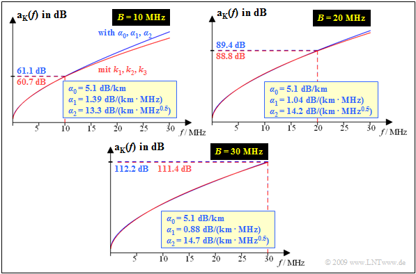
$\text{Example 2:}$  In the following graphs we assume the line length  $l = 1 \ \rm km$  and the diameter  $d = 0.4 \ \rm mm$,  so that the following applies:

Approximation of  $k$–parameters  by  $\alpha$–parameters

$$k_1 = 5.1 \ \rm dB/km, \ k_2 = 14.3 \ \rm dB/km, \ k_3 = \ 0.59.$$

For this case the following graph shows

• the attenuation approximated  ${\rm a_K}(f)$  (in dB)  with  $α_0,  α_1$,  $α_2$ 
  (blue curve)
• compared to the   ${\rm a_K}(f)$  curve according to  $k_1,  k_2,  k_3$ 
  (red curve).

The three diagrams are valid for the bandwidths  $B = 10 \ \rm MHz$,  $B = 20 \ \rm MHz$  and  $B = \ \rm 30 \ MHz$.

• The determined coefficients  $α_1$  and  $α_2$  are indicated.
•  $α_0 = k_1 = 5.1 \ \rm dB/km$  is always valid.

One recognizes from these representations:

• Even with the largest approximation range  $(B = 30 \ \rm MHz)$,  the blue curve  $($with  $α_0, \ α_1, \ α_2)$  approximates the measured curve  $($red curve,  described by  $k_1, \ k_2, \ k_3)$  very well.
• For smaller bandwidth  $(B = 20 \ \rm MHz$  or  $B = 10 \ \rm MHz)$  the approximation in the range  $0≤ f ≤ B$  is even better,  but then distortions occur for  $f > B$ .
• The attenuation value  $a_{\rm K}(f = 30 \ \rm MHz) ≈ 112.2 \ \rm dB$  is composed as follows for the considered two-wire cable:
      $4.5\%$  is due to the coefficient  $α_0$  (ohmic losses) ,  $23.5\%$  to the  $f$–proportional component  $α_1$  and  $72\%$  to the coefficient  $α_2$.
• In comparison, the standard  $\text{2.6/9.5 mm}$  coaxial cable exhibits comparable attenuation  $(≈ 112 \ \rm dB)$  only at a length of  $l = 8.7 \ \rm km$,  with most of the attenuation  $(98.9\%)$  coming from the skin effect  $(α_2)$.

In the opposite direction  $(α_1, \ α_2 ⇒ k_2, \ k_3)$  the conversion rule for the exponent is:

$$k_3 = \frac{H + 0.5} {H +1}, \hspace{0.4cm}\text{with auxiliary: }H = \frac{2} {3} \cdot \frac{\alpha_1 \cdot \sqrt{f_0}}{\alpha_2} \cdot \sqrt{B/f_0}.$$

With this result,  $k_2$  can be calculated using either of the two equations given above.

Impulse response of a two-wire line

With this coefficient conversion  $(k_1, \ k_2, \ k_3) \ \ ⇒ \ \ (α_0, \ α_1, \ α_2)$  we can now write for the total frequency response of a two-wire line:

$$H_{\rm K}(f) = H_{\alpha 0}(f) \cdot H_{\alpha 1}(f) \cdot H_{\beta 1}(f)\cdot H_{\alpha 2}(f) \cdot H_{\beta 2}(f) \hspace{0.05cm}.$$

Here,  the following abbreviations are used:

$$\begin{align*} H_{\alpha 0}(f) & = {\rm e}^{-\alpha_0 \hspace{0.05cm} \cdot \hspace{0.05cm} l}= {\rm e}^{-{\rm a}_0}\hspace{0.05cm},\hspace{0.2cm} {\rm a}_0= \alpha_0\hspace{0.15cm}{\rm (in \hspace{0.15cm}Np) }\cdot l,\\ H_{\alpha 1}(f) & = {\rm e}^{-\alpha_1 \cdot f \hspace{0.05cm} \cdot \hspace{0.05cm}l}= {\rm e}^{-{\rm a}_1 \cdot 2f/R}\hspace{0.05cm},\hspace{0.2cm} {\rm a}_1 = \alpha_1\hspace{0.15cm}{\rm (in \hspace{0.15cm}Np) }\cdot l \cdot {R}/{2} \hspace{0.05cm}, \\ H_{\beta 1}(f) & = {\rm e}^{-{\rm j} \hspace{0.05cm} \cdot \hspace{0.05cm} \beta_1 \cdot f \hspace{0.05cm} \cdot \hspace{0.05cm}l} = {\rm e}^{-{\rm j} \hspace{0.05cm} \cdot \hspace{0.05cm} 2 \pi \cdot f \hspace{0.05cm} \cdot \hspace{0.05cm}\tau_{\rm P}} \hspace{0.05cm},\hspace{0.2cm} \tau_{\rm P} = {\beta_1\hspace{0.15cm}{\rm (in \hspace{0.15cm}rad) }\cdot l }/({2 \pi}) \hspace{0.05cm}, \\ H_{\alpha 2}(f) & = {\rm e}^{-\alpha_2 \hspace{0.05cm}\cdot \hspace{0.05cm}\sqrt{f} \hspace{0.05cm} \cdot \hspace{0.05cm}l}= {\rm e}^{-{\rm a}_2 \hspace{0.05cm}\cdot \hspace{0.05cm}\sqrt{2f/R}}\hspace{0.05cm},\hspace{0.2cm} {\rm a}_2 = \alpha_2\hspace{0.15cm}{\rm (in \hspace{0.15cm}Np) }\cdot l \cdot \sqrt{R/2} \hspace{0.05cm}, \\ H_{\beta 2}(f) & = {\rm e}^{-{\rm j} \hspace{0.05cm} \cdot \hspace{0.05cm}\beta_2 \hspace{0.05cm} \cdot \hspace{0.05cm}\sqrt{f} \hspace{0.05cm} \cdot \hspace{0.05cm}l}= {\rm e}^{-{\rm j} \hspace{0.05cm} \cdot \hspace{0.05cm} b_2 \hspace{0.05cm}\cdot \hspace{0.05cm}\sqrt{2f/R}}\hspace{0.05cm},\hspace{0.2cm} b_2 = \beta_2\hspace{0.15cm}{\rm (in \hspace{0.15cm}rad) }\cdot l \cdot \sqrt{R/2} \hspace{0.05cm} \end{align*}$$

The meaning of the quantities implicitly defined here will be discussed a little later.

We proceed quite formally here first.  According to the  convolution theorem,  the resulting impulse response is the  Fourier retransform  of  $H_{\rm K}(f)$:

$$h_{\rm K}(t) = h_{\alpha 0}(t) \star h_{\alpha 1}(t) \star h_{\beta 1}(t)\star h_{\alpha 2}(t) \star h_{\beta 2}(t) \hspace{0.05cm},$$

$$h_{\alpha 0}(t) \quad \circ\!\!-\!\!\!-\!\!\!-\!\!\bullet\quad H_{\alpha 0}(f) \hspace{0.05cm},\hspace{0.2cm} h_{\alpha 1}(t) \circ\!\!-\!\!\!-\!\!\!-\!\!\bullet\quad H_{\alpha 1}(f) \hspace{0.05cm},\hspace{0.2cm} {\rm etc.}$$

These five components are now to be considered separately, with the numerical results referring to

• a digital transmission system with bit rate  $R = 30 \ \rm Mbit/s$  and
• a two-wire line with dimensions  $d = 0.4 \ \rm mm$  and  $l = 1 \ \rm km$. 

Thus,  the  $α$–coefficients in Neper  (Np) are:

$$\alpha_0 = 0.59\, \frac{ {\rm Np} }{ {\rm km} } \hspace{0.05cm}, \hspace{0.2cm} \alpha_1 = 0.10\, \frac{ {\rm Np} }{ {\rm km \cdot MHz} }\hspace{0.05cm}, \hspace{0.2cm} \alpha_2 = 1.69\, \frac{ {\rm Np} }{ {\rm km \cdot \sqrt{MHz} } } \hspace{0.05cm}.$$

The phase function per unit length of this line is also given in  [PW95]:

$$b_{\rm K}(f) = \beta_1 \cdot f + \beta_2 \cdot \sqrt {f}\hspace{0.05cm}, \hspace{0.2cm} \beta_1 = 32.9\, \frac{ {\rm rad} }{ {\rm km \cdot MHz} }\hspace{0.05cm}, \hspace{0.2cm} \beta_2 = 2.26\, \frac{ {\rm rad} }{ {\rm km \cdot \sqrt{MHz} } }\hspace{0.05cm}.$$

The symbol duration  $T = 1/R ≈ 33 \ \rm ns$  is suitable as a normalization quantity of time.

Interpretation and manipulation of the individual impulse responses

Now the five impulse response components  $h_{α0}(t), \ h_{α1}(t), \ h_{α2}(t), \ h_{β1}(t)$  and  $h_{β2}(t)$  are interpreted:

(1)   The first term resulting from the ohmic losses  (frequency-independent attenuation)  leads to a Dirac delta function with weight  $K$,  so that the convolution with  $h_{α0}(t)$  can be replaced by the multiplication with  $K = {\rm e}^{–0.59} ≈ 0.55$ :

$$h_{\alpha 0}(t) = K \cdot \delta(t) \hspace{0.25cm}{\rm with}\hspace{0.25cm} K = {\rm e}^{-{\rm a}_0}\hspace{0.45cm}\Rightarrow\hspace{0.45cm} h_{\rm K}(t) = h_{\alpha 0}(t) \star h_{\rm Rest}(t) = K \cdot h_{\rm Rest}(t)\hspace{0.05cm}.$$

(2)   $H_{α1}(f)$  is a real and even function of frequency,  so the Fourier retransform is also real and symmetric at  $t =0$:

$$H_{\alpha 1}(f) = {\rm e}^{-2\cdot{\rm a}_1 \cdot |f/R|} \quad \bullet\!\!-\!\!\!-\!\!\!-\!\!\circ\quad h_{\alpha 1}(t)= \frac{1}{T} \cdot \frac{{\rm a}_1}{{\rm a}_1^2 + \pi \cdot (t/T)^2}\hspace{0.05cm}, \hspace{0.2cm} {\rm a}_1 \hspace{0.15cm}{\rm in \hspace{0.15cm}Np } \hspace{0.05cm}.$$

With the exemplary numerical values  $α_1 = 0.1 \ \rm Np/(km · MHz)$,   $l = 1 \ \rm km$,   $R = 30 \ \rm MHz$   ⇒   ${\rm a}_1 = 1.5 \ \rm (Np)$,  we obtain for the maximum of this fraction:

$$h_{α1}(t = 0) = 1/{\rm a}_1 = 2/3 · 1/T.$$

(3)   As for the coaxial cable systems,  $H_{β1}(f)$  does not lead to any signal distortion,  but only to a time delay by the  phase delay time:

$$τ_{\rm P} ≈ 5.24 \ \rm µs \hspace{0.2cm} ⇒ \hspace{0.2cm} τ_{\rm P}/T ≈ 157.$$

(4)   Let us turn to the combined consideration of the  $H_{α2}(f)$  and  $H_{β2}(f)$  components,  which is described in the time domain by the partial impulse response  $h_2(t)$:

$$H_{\alpha 2}(f) \cdot H_{\beta 2}(f) \quad \bullet\!\!-\!\!\!-\!\!\!-\!\!\circ\quad h_{2}(t) \hspace{0.05cm}.$$

(5)   To apply the results of the chapter  Properties of Coaxial Cables,  we replace  $β_2$  by  $α_2 · \rm rad/Np$  and  $b_2$  by  ${\rm a}_2 · \text{rad/Np}$,  so that  ${\rm a}_2$  and  $b_2$  have the same numerical value.  As an example, we substitute here:

$$ b_2 = 8.75\, {\rm rad}\hspace{0.2cm} \Rightarrow \hspace{0.2cm} b_2 = 6.55 \,{\rm rad}\hspace{0.05cm}.$$

One thus reduces the constant  $β_2 = 2.26 \ \rm rad/(km · \sqrt{MHz})$  to  $β_2 = 1.69 \ \rm rad/(km · \sqrt{MHz})$ .

(6)   Before we unnecessarily lead the reader to consider whether this approximation is indeed valid or not,  we freely admit right away that this assumption is the weak point of our reasoning.  A discussion of this faulty assumption follows in the  next secction.

(7)   Now that  ${\rm a}_2$  and  $b_2$  have the same numerical values,  we can further use the equation given in the chapter  Properties of Coaxial Cables,  substituting  $\rm a_∗$  for  $\rm a_2$ :

$$h_{\rm 2}(t ) = \frac {1/T \cdot {\rm a_2}}{\pi \cdot \sqrt{2 \cdot(t/T)^3}}\cdot {\rm e}^{ - {{\rm a_2}^2}/( {2\pi \hspace{0.05cm}\cdot \hspace{0.05cm} t/T})} \hspace{0.05cm}, \hspace{0.2cm} {\rm a}_2\hspace{0.15cm}{\rm in \hspace{0.15cm}Np} \hspace{0.05cm}.$$

(8)   The total impulse response without consideration of the phase delay time is thus given by

$$h_{\rm K}(t + \tau_{\rm P}) = K \cdot h_{\alpha 1}(t) \star h_{2}(t)\hspace{0.05cm}.$$

By shifting  $τ_{\rm P}$  to the right, the searched function  $h_{\rm K}(t)$  is obtained.  In the following example,  this procedure is illustrated by graphics.

$\text{Example 3:}$  For the following graphs,  a two-wire line with dimensions  $d = 0.4 \ \rm mm$  and  $l = 1 \ \rm km$  is still assumed. Please note the different ordinate scaling of the three diagrams in the graph.

• The bit rate is  $R = 30 \ \rm Mbit/s$   ⇒   symbol duration  $T ≈ 33\ \rm ns$.
• We assume the quantities given in the yellow box,  calculated on the last page.
• For this purpose,  the  $b_2$ value is changed from  $8.75 \ \rm rad$  to  $6.55 \ \rm rad$  to match the  ${\rm a}_2$ value.
• The effects of this measure are interpreted on the next page.

For calculating the impulse response of a two-wire line

On the top right  $h_1(t) = h_{\rm α1}(t + τ_{\rm P})$  is shown. This component is due to the  $α_1$  and  $β_1$  coefficients. $h_1(t)$  is a symmetric function with respect to the phase delay time  $τ_{\rm P}$  with the maximum value  $(1.5T)^{–1}$, where the  $1/(1 + t^2$) decay is rapidly decreased at  $ \pm 5T$  $($right and left of  $τ_{\rm P})$.

The lower left diagram shows the signal component  $h_2(t)$,  due to the two coefficients  $α_2$  and  $β_2$.  $h_2(t)$  is identical to the  coaxial cable impulse response  (ignoring the delay time)  when the characteristic cable attenuation is  $6.55 \ \rm Np$  or  $56.9 \ \rm dB$.

The red curve represents the convolution product  $h_1(t) ∗ h_2(t)$.  It can be seen that the waveform is essentially fixed by  $h_2(t)$.  However,  convolution with  $h_1(t)$  leads to a  (slight)  distortion of the waveform in addition to an amplitude loss of about  $10\%$.

The resulting impulse response  $h_{\rm K}(t)$  of the 0.4mm two-wire line is shown as a blue curve in the lower right diagram.  The difference to the convolution product  $h_1(t) ∗ h_2(t)$  drawn in red results from the influence of the DC signal attenuation $($coefficient  $α_0)$.

You can illustrate the presented method for arbitrary parameters (diameter, length, bit rate) with the (German language) interactive SWF applet

Zeitverhalten von Kupferkabeln  ⇒   "Time behavior of copper cables". 

Discussion of the approximate solution found

Impulse response approximations of normal coaxial cable (top)
and  0.4 mm  two-wire cable (bottom)

$\text{Example 4:}$  The following graph shows the (normalized) impulse responses  $T · h_{\rm K}(t)$  for two exemplary copper cables, namely

• for the   $\text{standard coaxial cable 2.6/9.5 mm}$  at  $\text{10.1 km}$  length (above), where:

$$a_0 = 0.016\,{\rm Np}\hspace{0.05cm}, \hspace{0.15cm} a_1 = 0.020\,{\rm Np}\hspace{0.05cm}, \hspace{0.15cm} a_2 = 6.177\,{\rm Np}\hspace{0.05cm}, $$

$$\tau_{ {\rm P} }/T = 350\hspace{0.05cm}, \hspace{0.15cm} b_2 = 6.177\,{\rm rad}\hspace{0.05cm};$$

• for the   $\text{0.4 mm two-wire line}$ with the length $\text{1.8 km}$ (below) with the parameters

$$a_0 = 1.057\,{\rm Np}\hspace{0.05cm}, \hspace{0.15cm} a_1 = 0.147\,{\rm Np}\hspace{0.05cm}, \hspace{0.15cm} a_2 = 6.177\,{\rm Np}\hspace{0.05cm}, $$

$$\tau_{ {\rm P} }/T = 94\hspace{0.05cm}, \hspace{0.15cm} b_2 = 8.260\,{\rm rad}\hspace{0.05cm}.$$

These values are valid for bit rate  $R = 10 \ \rm Mbit/s$   ⇒   time normalization  $T = 0.1 \ \rm µ s$.

• The two cable lengths were chosen to give exactly equal  $a_2$ parameters.
• For the two-wire cable,  the phase value  $b_2 ⇒ b_2\hspace{0.01cm}'$  was adjusted to give equal values for  $b_2\hspace{0.05cm}' = 6.177 \ \rm rad$  and  $a_2 = 6.177 \ \rm Np \ (≈ 53 \ dB)$  as for the coaxial cable.

The blue curves show the approximations when the  $a_0, \ a_1$ and  $b_1$ terms are neglected.  Due to the  $b_2 ⇒ b_2\hspace{0.01cm}'$  phase matching for the two-wire line,  the curves are nearly the same.  The maximum of about  $3.8\%$  is at about  $t/T = 4$  (different time scales in both diagrams!).

The red curves also take into account the  $a_0, \ a_1$ and  $b_1 $  terms.  The red curve of the coaxial cable is the actual (normalized) impulse response  $T · h_{\rm K}(t)$.

From these representations, one can further see:

• For the coaxial cable,  the  $a_0$ term and the  $a_1 $  term can be neglected.  The resulting relative error is only  $3.5\%$.
• However, the phase delay time  $τ_{\rm P}$, i.e. the  $b_1$ term,  cannot be neglected.  For the coaxial cable this gives  $τ_{\rm P}/T ≈ 350$,  while for the two-wire line it is  $τ_{\rm P}/T ≈ 94$   (note the different time scales).
• For the two-wire line (below),  do not neglect DC signal attenuation  $(a_0)$  and transverse loss  $(a_1)$ :  
  The red approximation  $T · h_{\rm K}\hspace{0.01cm}'(t)$  is  $70\%$  lower than the blue one and also slightly wider.

$\text{Example 5:}$  This example shows approximations of the impulse response of a two-wire line  $($length $\text{1.8 km}$,  diameter $\text{0.4 mm)}$,  so that according to  [PW95]  the following parameters can be assumed:

For the impulse response of a  $\text{0.4 mm}$  two-wire cable

$$a_0 = 1.057\,{\rm Np}\hspace{0.05cm}, \hspace{0.15cm} a_1 = 0.147\,{\rm Np}\hspace{0.05cm}, \hspace{0.15cm} a_2 = 6.177\,{\rm Np}\hspace{0.05cm}, $$

$$\tau_{ {\rm P} }/T = 94\hspace{0.05cm}, \hspace{0.15cm} b_2 = 8.260\,{\rm rad}\hspace{0.05cm}.$$

The upper diagram – equal to the lower diagram in  $\text{Example 4}$ – shows two approximations

• with neglection of the  $a_0, \ a_1$  and  $b_1$ terms  (blue curve),
• with consideration of the  $a_0, \ a_1$  and  $b_1$ terms  (red curve).

For this upper diagram, we further adopted the  $a_2$ coefficient given in [PW95] and lowered the mentioned coefficient  $b_2 = 8.260 \ \rm rad$  to  $b_2\hspace{0.01cm}' = 6.177 \ \rm rad$ .

Note:   In contrast to the coaxial cable in  $\text{Example 3}$,  because of  $b_2\hspace{0.01cm}' ≠ b_2$  the red curve  $T · h_{\rm K}\hspace{0.01cm}'(t)$  is also only an approximation, which is indicated in the graphic by the apostrophe.

Without the correction  $b_2\hspace{0.01cm}' = a_2 · \text{rad/Np}$,  the  Hilbert Transformation, which establishes the relationship between magnitude and phase in real and thus establishes  minimum-phase systems,  would not be satisfied.  Therefore,  it would result in a noncausal impulse response.

We therefore believe that even for a two-wire line, the two parameters  $a_2$  and  $b_2$  should have equal numerical values.

We now consider a second approach,  shown in the diagram below:

• Here,  the phase coefficient  $b_2 = 8.260 \ \rm rad$  given in  [PW95]  was kept.
• Instead,  the attenuation coefficient  $a_2 = 6.177 \ \rm Np$  was adjusted to the phase coefficient (i.e., enlarged):   $a_2\hspace{0.01cm}' = 8.260 \ \rm Np$.
• The lower  (red)  impulse response   ⇒   "worst case"  is less than half as high and much wider than the upper impulse response   ⇒   "best case".
• The actual  (normalized)  impulse response  $T \cdot h_{\rm K}\hspace{0.01cm}'(t)$  will probably lie in between.  We do not allow ourselves to make more precise statements.

Crosstalk on two-wire lines

For transmission systems over two-wire lines,  the same  block diagram  can be assumed as for the coaxial cable systems,  where now

• for the frequency response  $H_{\rm K}(f)$  and the impulse response  $h_{\rm K}(t)$  the equations given in this section are to be used,
• white Gaussian noise  $N_0$  is no longer the dominant cause of stochastic impairments,  but  crosstalk  due to capacitive or inductive coupling of adjacent pairs now predominates.

By twisting the wire pairs of a star quad as well as the basic and main bundles according to the diagram at the end of the chapter  Access network of a telecommunications system  an attempt is made to achieve on average a mutual coupling as symmetrical as possible between all wire pairs.  Due to unavoidable manufacturing tolerances,  however,  a slight asymmetry always remains.  This causes

• in addition to its  "own"  useful signal,  each receiver input also receives  (usually only small)  signal components from neighboring wire pairs,
• the induced signal components represent an additional stochastic impairment for the useful signal,  which together with the thermal noise results in the resulting interfering signal  $n(t)$,
• the transmission quality cannot be improved or can only be improved to a very limited extent by increasing the transmitting power,  since this measure also increases the crosstalk interference.

To clarify near-end crosstalk (NEXT) and far-end crosstalk (FEXT)

As the diagram illustrates, a distinction is made between

• Near-End Crosstalk  $\rm (NEXT)$:
  The interfering transmitter feeds its signal at the same end of the cable where the receiver under consideration is placed.

• Far–End–Crosstalk  $\rm (FEXT)$:
  The interfering transmitter and the interfering receiver are located at opposite ends of the cable.

In the case of  "FEXT",  the interference accumulates over the entire cable length,  but is also greatly attenuated by the cable attenuation.  For bundled cables in the local loop area,  "in quad crosstalk"  thus results in orders of magnitude greater interference than long-distance crosstalk,  and even near-end crosstalk interference from adjacent cores can usually be neglected.

$\text{Without derivation:}$  We therefore consider only  $\text{Near-End Crosstalk (NEXT)}$  in the following.  In this case, the  power density spectrum  $\rm (PDS)$  of the interference signal  $n(t)$  can be represented as follows, taking into account the unavoidable thermal noise  $(N_0/2)$ :

$${\it \Phi}_n(f) = {N_0}/{2}+{\it \Phi}_{\rm NEXT}(f) \hspace{0.05cm},\hspace{0.3cm}{\rm with} \hspace{0.3cm}{\it \Phi}_{\rm NEXT}(f) = {\it \Phi}_{s}(f) \cdot\vert H_{\rm NEXT}(f)\vert ^2 \approx {\it \Phi}_{s}(f) \cdot [K_{\rm NEXT} \cdot f]^{3/2}\hspace{0.05cm}.$$

It should be noted about this equation:

• The equation is obtained by integrating the local couplings over the entire length of a short section,  where the couplings between all copper lines are modeled by cross capacitances and inductances.
• ${\it \Phi}_s(f)$  is the PDS of the interfering transmitter,  from which the transmission power  $P_{\rm S}$  is obtained by integration.  Assuming that the interfered transmission uses the same transmission signal and thus the same PDS  ${\it \Phi}_s(f)$  as the interferer,  it is clear that increasing  $P_{\rm S}$  only reduces the (relative) influence of thermal noise  $(N_0/2)$.
• The factor  $K_{\rm NEXT}$  quantifying the near-end crosstalk depends strongly on the core spacing,  as well as on the degree of unbalance along the cable.  In contrast,  this factor  $K_{\rm NEXT}$  is almost independent of the conductor diameter  $d$  and the cable length  $l$.
• The product  $K_{\rm NEXT} · f$  (dimensionless)  is always much smaller than  $1$  over the entire operating range of the cable,  e.g. for all frequencies  $0 ≤ f ≤ 30 \ \rm MHz$.  The crosstalk interference increases sharply $($that is,  with exponent $1.5)$  with frequency.
• In  [PW95],  the following values are given after a series of measurements over forty pairs for the frequency  $f = 10 \ \rm MHz$   $($for  $f = 30 \ \rm MHz$  these values must still be multiplied by  $3^{3/2} ≈ 5.2)$:

• worst case:   $|H_{\rm NEXT}(f = 10 \ \rm MHz)|^2 ≈ 0.001$,
• Averaging over 40 cores:   $|H_{\rm NEXT}(f = \ \rm 10 MHz)|^2 ≈ 0.0004$.

• This values apply to  "in-four near-end crosstalk"  (interfering transmitter and interfering receiver in the same star quad).
• Near-end crosstalk interference between more distant cores exhibits the same frequency dependence, but is smaller than  "in-four near-end crosstalk":

• Near-end crosstalk between adjacent star quads by about  $5 \ \rm dB$,
• Near-end crosstalk between adjacent ground bundles by about  $10 \ \rm dB$,
• Near-end crosstalk between non-adjacent ground bundles by about  $25 \ \rm dB$.

$\text{Conclusion:}$ 

• In order to avoid or at least reduce such near-end crosstalk interference,  adjacent pairs of wires are often occupied by completely different signals  (analog telephony, ISDN, DSL or other broadband services)  which also use different frequency bands if possible.
• By clever selection of the twisted pairs,  adjacent cores can now be occupied with signals whose spectra overlap as little as possible,  thus reducing crosstalk interference.

Exercises for the chapter

Exercise 4.6: $k$-Parameters and $\alpha$-Parameters

Exercise 4.6Z: ISDN Supply Lines

Exercise 4.7: Copper Twin Wire 0.5 mm

Exercise 4.8: Near-end and Far-end Crosstalk Disorders