Exercise 1.4Z: Modified MS43 Code

• Return to book

Code table of the MMS43 code

For ISDN data transmission,  the MMS43 code is used in Germany and Belgium on the so-called  "$\rm U_{\rm K0}$"  interface  $($transmission path between the exchange and the NTBA$)$. 

The abbreviation  "MMS43"  stands for  "Modified Monitored Sum 4B3T".

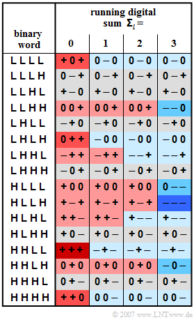
This is a 4B3T block code with the four code tables shown in the graphic,  which are used for coding according to the so-called "running digital sum"  $($after  $l$  blocks$)$:

$${\it \Sigma}\hspace{0.05cm}_l = \sum_{\nu = 1}^{3 \hspace{0.05cm}\cdot \hspace{0.05cm} l}\hspace{0.02cm} a_\nu$$

For initialization:  ${\it \Sigma}_{0} = 0$  is used.

The colorings in the graph mean:

• If the running digital sum does not change   $({\it \Sigma}\hspace{0.05cm}_{l+1} = {\it \Sigma}\hspace{0.05cm} _{l})$,  a field is grayed out.

• An increase   $({\it \Sigma}\hspace{0.05cm}_{l+1} > {\it \Sigma}\hspace{0.05cm}_{l})$   is highlighted in red,  a decrease   $({\it \Sigma}\hspace{0.05cm}_{l+1} < {\it \Sigma}\hspace{0.05cm} _{l})$   in blue.

• The more intense these colors are,  the greater the change in the running digital sum.

Notes:

• The exercise belongs to the chapter  "ISDN Basic Access".

• Information about the MMS43 code can be found in the chapter  "Block Coding with 4B3T Codes"  of the book  "Digital signal transmission".

Questions

1

What are the reasons for using the 4B3T code instead of the redundancy-free binary code in ISDN?

	4B3T is in principle better than the redundancy-free binary code.
	The transmitted signal should be free of DC signals if the channel frequency response  $H_{\rm K}(f = 0) = 0$.
	A small symbol rate  $(1/T)$  allows a longer cable length.

2

Encode the binary sequence  "$1100\hspace{0.08cm} 0100 \hspace{0.08cm} 0110 \hspace{0.08cm} 1010$"  according to the table.
What is the coefficient of the third ternary symbol of the fourth block?

$a_{12} \ = \ $

3

Determine the Markov diagram for the transition from  ${\it \Sigma}\hspace{0.05cm}_{l}$  to  ${\it \Sigma}\hspace{0.05cm}_{l+1}$.  What are the transition probabilities?

${\rm Pr}({\it \Sigma}\hspace{0.05cm}_{l+1} = 0 \ | \ {\it \Sigma}\hspace{0.05cm}_{l}=0) \ = \ $

${\rm Pr}({\it \Sigma}\hspace{0.05cm}_{l+1} = 2 \ | \ {\it \Sigma}\hspace{0.05cm}_{l}=0) \ = \ $

${\rm Pr}({\it \Sigma}\hspace{0.05cm}_{l+1} = 0 \ | \ {\it \Sigma}\hspace{0.05cm}_{l}=2) \ = \ $

4

What properties follow from the Markov diagram?

	The probabilities   ${\rm Pr}({\it \Sigma}\hspace{0.05cm}_{l} = 0), \text{ ...} \ , {\rm Pr}({\it \Sigma}\hspace{0.05cm}_{l} = 3)$   are equal.
	${\rm Pr}({\it \Sigma}\hspace{0.05cm}_{l} = 0) = {\rm Pr}({\it \Sigma}\hspace{0.05cm}_{l} = 3)$   and   ${\rm Pr}({\it \Sigma}\hspace{0.05cm}_{l} = 1) = {\rm Pr}({\it \Sigma}\hspace{0.05cm}_{l} = 2)$  are valid.
	The extreme values  $(0$ or $3)$  occur less frequently than  $1$  or  $2$.

Solution

Solution

(1)  Statements 2 and 3  are correct:

• The first statement is not true:  For example,  the AWGN channel  ("additive white Gaussian noise") with a 4B3T code results in a much larger error probability due to the ternary decision compared to the redundancy-free binary code.

• The essential reason for the use of a redundant transmission code is rather that no DC signal component can be transmitted via a  "telephone channel".

• The  $25 \%$  smaller symbol rate  $(1/T)$  of the 4B3T code also accommodates the transmission characteristics of copper lines  (strong increase in attenuation with frequency).

• For a given line attenuation,  therefore,  a greater length can be bridged with the 4B3T code than with a redundancy-free binary signal.

(2)  With the initial value  ${\it \Sigma}_{0} = 0$,  the 4B3T coding results in:

• 1100   ⇒   "+ + +"   ⇒   ${\it \Sigma}_{1} = 3$,

• 0100   ⇒   " – + 0"   ⇒   ${\it \Sigma}_{2} = 3$,

• 0110   ⇒   "– – +"   ⇒   ${\it \Sigma}_{3} = 2$,

• 1010   ⇒   "+ – –"   ⇒   ${\it \Sigma}_{4} = 1$.

Thus,  the amplitude coefficient we are looking for is  $a_{12}\hspace{0.15cm} \underline{ = \ –1}$.

Markov diagram for the MMS43 code

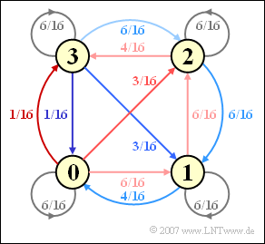
(3)  From the coloring of the given code table,  one can determine the following Markov diagram.

• From it,  the transition probabilities we are looking for can be read:

$${\rm Pr}({\it \Sigma}_{l+1} = 0 \ | \ {\it \Sigma}_{l}=0) \ = \ 6/16 \underline{ \ = \ 0.375},$$

$${\rm Pr}({\it \Sigma}_{l+1} = 2 \ | \ {\it \Sigma}_{l}=0) \ = \ 3/16 \underline{ \ = \ 0.1875},$$

$${\rm Pr}({\it \Sigma}_{l+1} = 0 \ | \ {\it \Sigma}_{l}=2) \underline{ \ = \ 0}.$$

(4)  Statements 2 and 3  are correct:

• The first statement is false,  which can be seen from the asymmetries in the Markov diagram.

• On the other hand,  there are symmetries with respect to the states  "0"  and  "3"  and between  "1"  and  "2".

In the following calculation,  instead of  ${\rm Pr}({\it \Sigma}_{l} = 0)$,  we write  ${\rm Pr}(0)$  in a simplified way.

• Taking advantage of the properties  ${\rm Pr}(3) = {\rm Pr}(0)$  and  ${\rm Pr}(2) = {\rm Pr}(1)$,  we get the following equations from the Markov diagram:

$${\rm Pr}(0)= \frac{6}{16} \cdot {\rm Pr}(0) + \frac{4}{16} \cdot {\rm Pr}(1)+ \frac{1}{16} \cdot {\rm Pr}(3)\hspace{0.3cm} \Rightarrow \hspace{0.3cm}\frac{9}{16} \cdot {\rm Pr}(0)= \frac{4}{16} \cdot {\rm Pr}(1).$$

• From the further condition  ${\rm Pr}(0) + {\rm Pr}(1) = 1/2$  follows further:

$${\rm Pr}(0)= {\rm Pr}(3)= \frac{9}{26}\hspace{0.05cm}, \hspace{0.2cm} {\rm Pr}(1)= {\rm Pr}(2)= \frac{4}{26}\hspace{0.05cm}.$$

This calculation is based on the  sum of the incoming arrows in the "0" condition.

• One could also give equations for the other three states,  but they all give the same result:

$${\rm Pr}(1) \ = \ \frac{6}{16} \cdot {\rm Pr}(0) + \frac{6}{16} \cdot {\rm Pr}(1)+ \frac{6}{16} \cdot {\rm Pr}(2)+\frac{3}{16} \cdot {\rm Pr}(3)\hspace{0.05cm},$$

$${\rm Pr}(2) \ = \ \frac{3}{16} \cdot {\rm Pr}(0) + \frac{6}{16} \cdot {\rm Pr}(1)+ \frac{6}{16} \cdot {\rm Pr}(2)+\frac{6}{16} \cdot {\rm Pr}(3)\hspace{0.05cm},$$

$${\rm Pr}(3) \ = \ \frac{1}{16} \cdot {\rm Pr}(0) + \frac{4}{16} \cdot {\rm Pr}(2)+\frac{6}{16} \cdot {\rm Pr}(3)\hspace{0.05cm}.$$