Exercise 4.3: Algebraic and Modulo Sum
From LNTwww
(Redirected from Aufgabe 4.3: Algebraische und Modulo-Summe)


A "clocked" random number generator returns a sequence $\langle x_\nu \rangle$ of binary random numbers.
- It is assumed that the binary numbers $0$ and $1$ occur with equal probabilities and that the individual random numbers do not depend on each other.
- The random numbers $ x_\nu \in \{0, 1\}$ are entered into the first memory location of a shift register and shifted down one digit with each clock pulse.
Two new random sequences $\langle a_\nu \rangle$ and $\langle m_\nu \rangle$ are formed from the contents of the three-digit shift register. Here denotes:
- the "algebraic sum" $a_\nu$:
- $$a_\nu=x_\nu+x_{\nu-1}+x_{\nu-2},$$
- the "modulo–2 sum" $m_\nu$:
- $$m_\nu=x_\nu\oplus x_{\nu-1}\oplus x_{\nu-2}.$$
Hints:
- This exercise belongs to the chapter Two-Dimensional Random Variables.
- Use the following table for moment calculation.
Questions
Solution
(1) It can be seen from the table in the information section that for the modulo–2 sum, the two values $0$ and $1$ have equal probability:
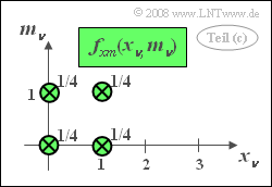
2D–PDF of $x$ and $m$ 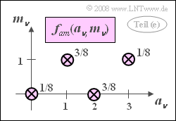
2D–PDF of $a$ and $m$
- $${\rm Pr}(m_\nu = 0) = {\rm Pr}(m_\nu = 1)\hspace{0.15cm}\underline{=0.5}.$$
(2) The table shows that for each preassignment ⇒ $( x_{\nu-1}, x_{\nu-2}) = (0,0), (0,1), (1,0), (1,1)$, the values $m_\nu = 0$ and $m_\nu = 1$ resp. are equally likely.
- Expressed differently: ${\rm Pr}(m_{\nu}\hspace{0.05cm}|\hspace{0.05cm}m_{\nu-1}) = {\rm Pr}( m_{\nu}).$
- This exactly matches the definition of "statistical independence" ⇒ Answer 1.

(3) Correct are the second and the last suggested solutions.
- The 2D–PDF consists of four Dirac delta functions, each with weight $1/4$.
- One obtains this result, for example, by evaluating the table in the data section.
- Since $f_{xm}(x_\nu, m_\nu)=f_{x}(x_\nu) \cdot f_{m}(m_\nu)$, the quantities $x_\nu$ and $m_\nu$ are statistically independent.
- Statistically independent random variables, however, are also linearly statistically independent, so they are certainly uncorrelated.
(4) Within the sequence $\langle a_\nu \rangle$ of algebraic sum there are statistical bindings ⇒ Answer 2.
- You can see this because the unconditional probability is $ {\rm Pr}( a_{\nu} = 0) =1/8$,
- while, for example, ${\rm Pr}(a_{\nu} = 0\hspace{0.05cm}|\hspace{0.05cm}a_{\nu-1} = 3) =0$ holds.

(5) Correct are the first and the last suggested solutions:
- As in the subtask (3) there are again four Dirac delta functions, but this time not with equal Dirac weights $1/4$.
- The two-dimensional PDF thus cannot be written as a product of the two marginal probability densities.
- But this means that statistical bindings must exist between $a_\nu$ and $m_\nu$.
- For the joint expected value, one obtains:
- $${\rm E}\big[a\cdot m \big] = \rm \frac{1}{8}\cdot 0 \cdot 0 +\frac{3}{8}\cdot 2 \cdot 0 +\frac{3}{8}\cdot 1 \cdot 1 + \frac{1}{8}\cdot 3 \cdot 1 = \frac{3}{4}.$$
- With the linear means ${\rm E}\big[a \big] = 1.5$ and ${\rm E}[m] = 0.5$ it follows for the covariance:
- $$\mu_{am}= {\rm E}\big[ a\cdot m \big] - {\rm E}\big[ a \big]\cdot {\rm E} \big[ m \big] = \rm 0.75-1.5\cdot 0.5 = \rm 0.$$
- Thus, the correlation coefficient $\rho_{am}= 0$. That is: The dependencies present are nonlinear.
- The quantities $a_\nu$ and $m_\nu$ are statistically dependent, but still uncorrelated.