Exercise 2.7: C Programs "z1" and "z2"

C programs for generating
discrete random variables

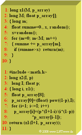
The two C programs given here are suitable for generating discrete random variables:

The function $z1$ generates an $M$–level random variable with the value set $\{0, 1$, ... , $M-1\}$. The associated probabilities are passed in the array $\text{p_array}$ with property "Float" The function $\text{random()}$ returns equally distributed float–random variables between $0$ and $1$.

A second function $z2$ (source code see below) returns a special probability distribution specified by the two parameters $I$ and $p$. This is done using the function $z1$.

Hints:

The exercise belongs to the chapter Generation of Discrete Random Variables.
In particular, reference is made to the page Generation of multilevel random variables.

Questions

$z1 \ = \ $

	You could omit the assignment $\text{x = random()}$ in line 5 and compare directly with $\text{random()}$ in line 8.
	If all probabilities passed to the function are equal, there would be faster program realizations than $z1$.
	The return value $\text{random() = 0.2}$ leads to the result $z1= 1$.

	The program generates a "binomially distributed random variable".
	The program generates a "Poisson distributed random variable".
	With $I = 4$ the values $0, \ 1, \ 2, \ 3, \ 4$ are possible for $z2$.
	The inclusion of the mathematical library "math.h" is required because in $z2$ the function "pow" ("exponentiate") is used in $z2$.

$\text{p_array[2]} \ = \ $

Solution

(1) After the first iteration of the loop $(m = 0)$ the variable $\text{sum = 0.2}$, at the next iteration $(m = 1)$ holds $\text{sum = 0.2 + 0.3 = 0.5}$.

In both cases: $\text{sum}$ is less than $x = 0.75$.
Only at $m = 2$ the return condition is satisfied: $0.9 > x$. Thus $\underline{z1 = 2}$.

(2) Correct are the solutions 2 and 3:

If one were to dispense with the auxiliary variable $x$ and write in line 8 instead "$\text{sum > random()}$" a new random value would be generated on each iteration of the loop, and $z1$ would then not have the desired properties.
$z1$ works according to the diagram on the page "Generation of multilevel random variables" in the theory section. There you find a faster implementation for the case of equal probabilities $(1/M)$.
In this case: In the first run $(m = 0)$ the return condition is not satisfied due to the "Lesser/Equal" query; the output value is actually $z1 = 1$.

(3) Correct are the solutions 1, 3, and 4:

It results in a binomially distributed random variable, with $z2 \in \{0, 1, 2, 3, 4\}$.
For the calculation of the probability ${\rm Pr}(z2 = 0) = (1 -p)^{I}$ one needs the mathematical library.
But exponentiation could also be realized by by multiplying $I$ times.

(4) Because of line 6, before the program loop $(i = 0)$ the field element $\text{p_array[0]}=(1 -p)^{I}$.

In the first iteration $(i = 1)$ the following value is entered:

$$\text{p_array[1]}=\frac{ p\cdot I}{ 1- p}\cdot\text{p_array[0]}= I\cdot p\cdot(1- p)^{ I- 1}={\rm Pr}(z2= 1) .$$

In the second iteration $(i = 2)$ the probability for the result "$z2=2$" is calculated:

$$\text{p_array[2]}=\frac{p\cdot (I- 1)}{ 2\cdot ( 1- p)}\cdot\text{p_array[1]}= \left({ I \atop { 2}}\right)\cdot p^{\rm 2}\cdot( 1- p)^{\rm 2}={\rm Pr}( z2 = 2) .$$

For $I= 4$ and $p = 0.25$ we get the following numerical value ⇒ "$4$ over $2$" $=6$:

$$\text{p_array[2]}={\rm Pr}( z 2=2)=6\cdot\frac{1}{16}\cdot\frac{9}{16} \hspace{0.15cm}\underline{=0.211}.$$