Exercise 3.5Z: Kullback-Leibler Distance again
The probability mass function is:
- $$P_X(X) = \big[\hspace{0.03cm}0.25\hspace{0.03cm}, \hspace{0.15cm} 0.25\hspace{0.15cm},\hspace{0.15cm} 0.25 \hspace{0.03cm}, \hspace{0.15cm} 0.25\hspace{0.03cm}\big]\hspace{0.05cm}.$$
The random variable $X$ is thus characterised by
- the symbol set size $M=4$,
- equal probabilities $P_X(1) = P_X(2) = P_X(3) = P_X(4) = 1/4$ .
The random variable $Y$ is always an approximation for $X$:
- It was obtained by simulation from a uniform distribution, whereby only $N$ random numbers were evaluated in each case. This means:
- $P_Y(1)$, ... , $P_Y(4)$ are not probabilities in the conventional sense. Rather, they describe relative frequencies.
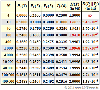
The result of the sixth test series (with $N=1000)$ is thus summarised by the following probability function:
- $$P_Y(X) = \big [\hspace{0.05cm}0.225\hspace{0.15cm}, \hspace{0.05cm} 0.253\hspace{0.05cm},\hspace{0.15cm} 0.250 \hspace{0.05cm}, \hspace{0.15cm} 0.272\hspace{0.05cm}\big] \hspace{0.05cm}.$$
This notation already takes into account that the random variables $X$ and $Y$ are based on the same alphabet $X = \{1,\ 2,\ 3,\ 4\}$.
With these preconditions, the informational divergence between the two probability functions $P_X(.)$ and $P_Y(.)$ :
- $$D(P_X \hspace{0.05cm}|| \hspace{0.05cm} P_Y) = {\rm E}_X \hspace{-0.1cm}\left [ {\rm log}_2 \hspace{0.1cm} \frac{P_X(X)}{P_Y(X)}\right ] \hspace{0.2cm}=\hspace{0.2cm} \sum_{\mu = 1}^{M} P_X(\mu) \cdot {\rm log}_2 \hspace{0.1cm} \frac{P_X(\mu)}{P_Y(\mu)} \hspace{0.05cm}.$$
One calls $D( P_X\hspace{0.05cm} || \hspace{0.05cm}P_Y)$ the (first) Kullback-Leibler distance.
- This is a measure of the similarity between the two probability mass functions $P_X(.)$ and $P_Y(.)$.
- The expected value formation occurs here with regard to the (actually equally distributed) random variable $X$. This is indicated by the nomenclature ${\rm E}_X\big[.\big]$.
A second form of Kullback-Leibler distance results from the formation of expected values with respect to the random variable $Y$ ⇒ ${\rm E}_Y\big [.\big ]$:
- $$D(P_Y \hspace{0.05cm}|| \hspace{0.05cm} P_X) = {\rm E}_Y \hspace{-0.1cm} \left [ {\rm log}_2 \hspace{0.1cm} \frac{P_Y(X)}{P_X(X)}\right ] \hspace{0.2cm}=\hspace{0.2cm} \sum_{\mu = 1}^M P_Y(\mu) \cdot {\rm log}_2 \hspace{0.1cm} \frac{P_Y(\mu)}{P_X(\mu)} \hspace{0.05cm}.$$
Hints:
- The exercise belongs to the chapter Some preliminary remarks on two-dimensional random variables.
- In particular, reference is made to the page Relative entropy – Kullback-Leibler distance.
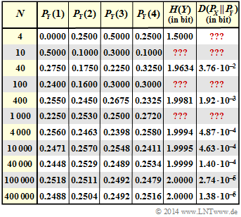
- The entropy $H(Y)$ and the Kullback-Leibler distance $D( P_X \hspace{0.05cm}|| \hspace{0.05cm}P_Y)$ in the above graph are to be understood in "bit".
- The fields marked with "???" in the graph are to be completed by you in this task.
Questions
Solution
(1) With equal probabilities, and with $M = 4$:
- $$H(X) = {\rm log}_2 \hspace{0.1cm} M \hspace{0.15cm} \underline {= 2\,{\rm (bit)}} \hspace{0.05cm}.$$
(2) The probabilities for the empirically determined random variables $Y$ generally (not always!) deviate from the uniform distribution the more the parameter $N$ is smaller. One obtains for
- $N = 1000 \ \ \Rightarrow \ \ P_Y(Y) = \big [0.225, \ 0.253, \ 0.250, \ 0.272 \big ]$:
- $$H(Y) = 0.225 \cdot {\rm log}_2 \hspace{0.1cm} \frac{1}{0.225} + 0.253 \cdot {\rm log}_2 \hspace{0.1cm} \frac{1}{0.253} + 0.250 \cdot {\rm log}_2 \hspace{0.1cm} \frac{1}{0.250} + 0.272 \cdot {\rm log}_2 \hspace{0.1cm} \frac{1}{0.272} \hspace{0.15cm} \underline {= 1.9968\ {\rm (bit)}} \hspace{0.05cm},$$
- $N = 100 \ \ \Rightarrow \ \ P_Y(Y) = \big[0.24, \ 0.16, \ 0.30, \ 0.30\big]$:
- $$H(Y) = \hspace{0.05cm}\text{...} \hspace{0.15cm} \underline {= 1.9410\ {\rm (bit)}} \hspace{0.05cm},$$
- $N = 10 \ \ \Rightarrow \ \ P_Y(Y) = \big[0.5, \ 0.1, \ 0.3, \ 0.1 \big]$:
- $$H(Y) = \hspace{0.05cm}\text{...} \hspace{0.15cm} \underline {= 1.6855\ {\rm (bit)}} \hspace{0.05cm}.$$
(3) The equation for the Kullback-Leibler distance we are looking for is:
- $$D(P_X \hspace{0.05cm}|| \hspace{0.05cm} P_Y) = \sum_{\mu = 1}^{4} P_X(\mu) \cdot {\rm log}_2 \hspace{0.1cm} \frac{P_X(\mu)}{P_Y(\mu)} = \frac{1/4}{{\rm lg} \hspace{0.1cm}(2)} \cdot \left [ {\rm lg} \hspace{0.1cm} \frac{0.25}{P_Y(1)} + \frac{0.25}{P_Y(2)} + \frac{0.25}{P_Y(3)} + \frac{0.25}{P_Y(4)} \right ] $$
- $$\Rightarrow \hspace{0.3cm} D(P_X \hspace{0.05cm}|| \hspace{0.05cm} P_Y) = \frac{1}{4 \cdot {\rm lg} \hspace{0.1cm}(2)} \cdot \left [ {\rm lg} \hspace{0.1cm} \frac{0.25^4}{P_Y(1) \cdot P_Y(2)\cdot P_Y(3)\cdot P_Y(4)} \right ] \hspace{0.05cm}.$$
The logarithm to the base $ 2$ ⇒ $\log_2(.)$ was replaced by the logarithm to the base $ 10$ ⇒ $\lg(.)$ for easy use of the calculator.
The following numerical results are obtained:
- for $N=1000$:
- $$D(P_X \hspace{0.05cm}|| \hspace{0.05cm} P_Y) = \frac{1}{4 \cdot {\rm lg} \hspace{0.1cm}(2)} \cdot \left [ {\rm lg} \hspace{0.1cm} \frac{0.25^4}{0.225 \cdot 0.253\cdot 0.250\cdot 0.272} \right ] \hspace{0.15cm} \underline {= 0.00328 \,{\rm (bit)}} \hspace{0.05cm},$$
- for $N=100$:
- $$D(P_X \hspace{0.05cm}|| \hspace{0.05cm} P_Y) = \frac{1}{4 \cdot {\rm lg} \hspace{0.1cm}(2)} \cdot \left [ {\rm lg} \hspace{0.1cm} \frac{0.25^4}{0.24 \cdot 0.16\cdot 0.30\cdot 0.30} \right ] \hspace{0.15cm} \underline {= 0.0442 \,{\rm (bit)}} \hspace{0.05cm},$$
- for $N=10$:
- $$D(P_X \hspace{0.05cm}|| \hspace{0.05cm} P_Y) = \frac{1}{4 \cdot {\rm lg} \hspace{0.1cm}(2)} \cdot \left [ {\rm lg} \hspace{0.1cm} \frac{0.25^4}{0.5 \cdot 0.1\cdot 0.3\cdot 0.1} \right ] \hspace{0.15cm} \underline {= 0.345 \,{\rm (bit)}} \hspace{0.05cm}.$$
(4) Correct is No, as will be shown by the example $N = 100$ :
- $$D(P_Y \hspace{0.05cm}|| \hspace{0.05cm} P_X) = \sum_{\mu = 1}^M P_Y(\mu) \cdot {\rm log}_2 \hspace{0.1cm} \frac{P_Y(\mu)}{P_X(\mu)} = 0.24\cdot {\rm log}_2 \hspace{0.1cm} \frac{0.24}{0.25} + 0.16\cdot {\rm log}_2 \hspace{0.1cm} \frac{0.16}{0.25} +2 \cdot 0.30\cdot {\rm log}_2 \hspace{0.1cm} \frac{0.30}{0.25} = 0.0407\ {\rm (bit)}\hspace{0.05cm}.$$
- In subtask (3) we got $D(P_X\hspace{0.05cm}|| \hspace{0.05cm} P_Y) = 0.0442$ instead.
- This also means: The designation „distance” is somewhat misleading.
- According to this, one would actually expect $D(P_Y\hspace{0.05cm}|| \hspace{0.05cm} P_X) = D(P_X\hspace{0.05cm}|| \hspace{0.05cm} P_Y)$ .
(5) With $P_Y(X) = \big [0, \ 0.25, \ 0.5, \ 0.25 \big ]$ one obtains:
- $$D(P_X \hspace{0.05cm}|| \hspace{0.05cm} P_Y) = 0.25\cdot {\rm log}_2 \hspace{0.1cm} \frac{0.25}{0} + 2 \cdot 0.25\cdot {\rm log}_2 \hspace{0.1cm} \frac{0.25}{0.25}+0.25\cdot {\rm log}_2 \hspace{0.1cm} \frac{0.25}{0.50}\hspace{0.05cm}.$$
- Because of the first term, the value of $D(P_X\hspace{0.05cm}|| \hspace{0.05cm}P_Y)$ is infinitely large.
- For the second Kullback-Leibler distance holds:
- $$D(P_Y \hspace{0.05cm}|| \hspace{0.05cm} P_X) = 0\cdot {\rm log}_2 \hspace{0.1cm} \frac{0}{0.25} + 2 \cdot 0.25\cdot {\rm log}_2 \hspace{0.1cm} \frac{0.25}{0.25}+ 0.50\cdot {\rm log}_2 \hspace{0.1cm} \frac{0.5}{0.25} \hspace{0.05cm}.$$
- After looking at the limits, one can see that the first term yields the result $0$ . The second term also yields zero, and one obtains as the final result:
- $$D(P_Y \hspace{0.05cm}|| \hspace{0.05cm} P_X) = 0.50\cdot {\rm log}_2 \hspace{0.1cm} (2) \hspace{0.15cm} \underline {= 0.5\,{\rm (bit)}} \hspace{0.05cm}.$$
Statements 3 and 5 are therefore correct:
- From this extreme example it is clear that $D(P_Y\hspace{0.05cm}|| \hspace{0.05cm} P_X)$ is always different from $D(P_X\hspace{0.05cm}|| \hspace{0.05cm} P_Y)$ .
- Only for the special case $P_Y \equiv P_X$ are both Kullback-Leibler distances equal, namely zero.
- The adjacent table shows the complete result of this task.
(6) Correct is again No. Although the tendency is clear: The larger $N$ is,
- the more $H(Y)$ approaches in principle the final value $H(X) = 2 \ \rm bit$,
- the smaller the distances $D(P_X\hspace{0.05cm}|| \hspace{0.05cm} P_Y)$ and $D(P_Y\hspace{0.05cm}|| \hspace{0.05cm} P_X)$ become.
However, one can also see from the table that there are exceptions:
- The entropy $H(Y)$ is smaller for $N = 1000$ than for $N = 400$.
- The distance $D(P_X\hspace{0.05cm}|| \hspace{0.05cm}P_Y)$ is greater for $N = 1000$ than for $N = 400$.
- The reason for this is that the experiment documented here with $N = 400$ was more likely to lead to a uniform distribution than the experiment with $N = 1000$.
- If, on the other hand, one were to start a very (infinitely) large number of experiments with $N = 400$ and $N = 1000$ and average over all of them, the actually expected monotonic course would actually result.

