Exercise 4.3: PDF Comparison with Regard to Differential Entropy
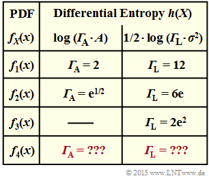
The adjacent table shows the comparison result with respect to the differential entropy $h(X)$ for
- the uniform distribution ⇒ $f_X(x) = f_1(x)$:
- $$f_1(x) = \left\{ \begin{array}{c} 1/(2A) \\ 0 \\ \end{array} \right. \begin{array}{*{20}c} {\rm{f\ddot{u}r}} \hspace{0.1cm} |x| \le A \\ {\rm else} \\ \end{array} ,$$
- the triangular distribution ⇒ $f_X(x) = f_2(x)$:
- $$f_2(x) = \left\{ \begin{array}{c} 1/A \cdot \big [1 - |x|/A \big ] \\ 0 \\ \end{array} \right. \begin{array}{*{20}c} {\rm{f\ddot{u}r}} \hspace{0.1cm} |x| \le A \\ {\rm else} \\ \end{array} ,$$
- the Laplace distribution ⇒ $f_X(x) = f_3(x)$:
- $$f_3(x) = \lambda/2 \cdot {\rm e}^{-\lambda \hspace{0.05cm} \cdot \hspace{0.05cm}|x|}\hspace{0.05cm}.$$
The values for the Gaussian distribution ⇒ $f_X(x) = f_4(x)$ with
- $$f_4(x) = \frac{1}{\sqrt{2\pi \sigma^2}} \cdot {\rm e}^{ - \hspace{0.05cm}{x ^2}/{(2 \sigma^2})}$$
are not yet entered here. These are to be determined in subtasks (1) to (3) .
Each probability density function $\rm (PDF)$ considered here is
- symmetric about $x = 0$ ⇒ $f_X(-x) = f_X(x)$
- and thus zero mean ⇒ $m_1 = 0$.
In all cases considered here, the differential entropy can be represented as follows:
- Under the constraint $|X| ≤ A$ ⇒ peak constraint $($German: "Spitzenwertbegrenzung" or "Amplitudenbegrenzung" ⇒ Identifier: $\rm A)$:
- $$h(X) = {\rm log} \hspace{0.1cm} ({\it \Gamma}_{\hspace{-0.01cm}\rm A} \cdot A) \hspace{0.05cm},$$
- Under the constraint ${\rm E}\big [|X – m_1|^2 \big ] ≤ σ^2$ ⇒ power constraint $($German: "Leistungsbegrenzung" ⇒ Identifier: $\rm L)$:
- $$h(X) = {1}/{2} \cdot {\rm log} \hspace{0.1cm} ({\it \Gamma}_{\hspace{-0.01cm}\rm L} \cdot \sigma^2) \hspace{0.05cm}.$$
The larger the respective parameter ${\it \Gamma}_{\hspace{-0.01cm}\rm A}$ or ${\it \Gamma}_{\hspace{-0.01cm}\rm L}$ is, the more favorable is the present PDF in terms of differential entropy for the agreed constraint.
Hints:
- The exercise belongs to the chapter Differential Entropy.
- Useful hints for solving this task can be found in particular on the pages
Questions
Solution
- $$f_X(x) = f_4(x) =A \cdot {\rm exp} [ - \hspace{0.05cm}\frac{x ^2}{2 \sigma^2}] \hspace{0.5cm}{\rm with}\hspace{0.5cm} A = \frac{1}{\sqrt{2\pi \sigma^2}}\hspace{0.05cm}.$$
- Logarithmizing this function, the result is proposed solution 1:
- $${\rm ln}\hspace{0.1cm} \big [f_X(x) \big ] = {\rm ln}\hspace{0.1cm}(A) + {\rm ln}\hspace{0.1cm}\left [{\rm exp} ( - \hspace{0.05cm}\frac{x ^2}{2 \sigma^2}) \right ] = {\rm ln}\hspace{0.1cm}(A) - \frac{x ^2}{2 \sigma^2}\hspace{0.05cm}.$$
(2) Both proposed solutions are correct:
- Using the result from (1) we obtain for the differential entropy in "nat":
- $$h_{\rm nat}(X)= -\hspace{-0.1cm} \int_{-\infty}^{+\infty} \hspace{-0.15cm} f_X(x) \cdot {\rm ln} \hspace{0.1cm} [f_X(x)] \hspace{0.1cm}{\rm d}x = - {\rm ln}\hspace{0.1cm}(A) \cdot \int_{-\infty}^{+\infty} \hspace{-0.15cm} f_X(x) \hspace{0.1cm}{\rm d}x + \frac{1}{2 \sigma^2} \cdot \int_{-\infty}^{+\infty} \hspace{-0.15cm} x^2 \cdot f_X(x) \hspace{0.1cm}{\rm d}x = - {\rm ln}\hspace{0.1cm}(A) + {1}/{2} \hspace{0.05cm}.$$
- Here it is taken into account that the first integral is equal to $1$ (PDF area).
- The second integral also gives the variance $\sigma^2$ (if, as here, the equal part $m_1 = 0$ ).
- Substituting the abbreviation variable $A$, we obtain:
- $$h_{\rm nat}(X) \hspace{-0.15cm} = \hspace{-0.15cm} - {\rm ln}\hspace{0.05cm}\left (\frac{1}{\sqrt{2\pi \sigma^2}} \right ) + {1}/{2} = {1}/{2}\cdot {\rm ln}\hspace{0.05cm}\left ({2\pi \sigma^2} \right ) + {1}/{2} \cdot {\rm ln}\hspace{0.05cm}\left ( {\rm e} \right ) = {1}/{2} \cdot {\rm ln}\hspace{0.05cm}\left ({{2\pi {\rm e} \cdot \sigma^2}} \right ) \hspace{0.05cm}.$$
- If the differential entropy $h(X)$ is not to be given in "nat" but in "bit", choose base $2$ for the logarithm:
- $$h_{\rm bit}(X) = {1}/{2} \cdot {\rm log}_2\hspace{0.05cm}\left ({{2\pi {\rm e} \cdot \sigma^2}} \right ) \hspace{0.05cm}.$$
(3) Thus, according to the implicit definition $h(X) = {1}/{2} \cdot {\rm log} \hspace{0.1cm} ({\it \Gamma}_{\hspace{-0.01cm}\rm L} \cdot \sigma^2)$ , the parameter is:
- $${\it \Gamma}_{\rm L} = 2\pi {\rm e} \hspace{0.15cm}\underline{\approx 17.08} \hspace{0.05cm}.$$
(4) We now consider a Gaussian probability density function with mean $m_1$:
- $$f_X(x) = \frac{1}{\sqrt{2\pi \sigma^2}} \cdot {\rm exp}\left [ - \hspace{0.05cm}\frac{(x -m_1)^2}{2 \sigma^2} \right ] \hspace{0.05cm}.$$
- The second moment $m_2 = {\rm E}\big [X ^2 \big ]$ can also be called the power $P$, while for the variance holds (this is also the second central moment):
- $$\sigma^2 = {\rm E}\big [|X – m_1|^2 \big ] = \mu_2.$$
- According to Steiner's theorem, $P = m_2 = m_1^2 + \sigma^2$. Thus, assuming $m_1 = \sigma = 1$ ⇒ $\underline{P/\sigma^2 = 2}$.
- Due to the DC component, the power is indeed doubled. However, this does not change anything in the differential entropy. Thus, it is still valid:
- $$h(X) = {1}/{2} \cdot {\rm log}_2\hspace{0.05cm}\left ({{2\pi {\rm e} \cdot \sigma^2}} \right )= {1}/{2} \cdot {\rm log}_2\hspace{0.05cm} (17.08)\hspace{0.15cm}\underline{\approx 2.047\,{\rm bit}} \hspace{0.05cm}.$$
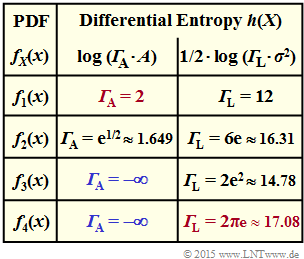
(5) Correct are the proposed solutions (1) and (4). The numerical values of the characteristics ${\it \Gamma}_{\rm L}$ and ${\it \Gamma}_{\rm A}$ are also entered in the completed table on the right.
A probability density function $f_X(x)$ is always particularly favorable under power constraints if the value ${\it \Gamma}_{\rm L}$ (right column) is as large as possible. Then the differential entropy $h(X)$ is also large.
The numerical results can be interpreted as follows:
- As is proved in the theory part, the Gaussian PDF $f_4(x)$ leads here to the largest possible ${\it \Gamma}_{\rm L} ≈ 17.08$ ⇒ the proposed solution 1 is correct (the value in the last column is marked in red).
- For the uniform PDF $f_1(x)$ the parameter ${\it \Gamma}_{\rm L} = 12$ is the smallest in the whole table ⇒ the proposed solution 2 is wrong.
- The triangular PDF $f_2(x)$ with ${\it \Gamma}_{\rm L} = 16.31$ is more favorable than the uniform PDF ⇒ the proposed solution 3 is wrong.
- The triangular PDF $f_2(x)$ is also better than the Laplace PDF $f_2(x) \ \ ({\it \Gamma}_{\rm L} = 14.78)$ ⇒ the proposed solution 4 is correct.
(6) Correct is the proposed solution (2). A PDF $f_X(x)$ is favorable in terms of differential entropy $h(X)$ under the peak constraint ⇒ $|X| ≤ A$, if the weighting factor ${\it \Gamma}_{\rm A}$ (middle column) is as large as possible:
- As shown in the theory section, the uniform distribution $f_1(x)$ leads here to the largest possible ${\it \Gamma}_{\rm A}= 2$ ⇒ the proposed solution 2 is correct (the value in the middle column is marked in red).
- The triangular PDF $f_2(x)$, which is also peak-constrained, is characterized by a somewhat smaller ${\it \Gamma}_{\rm A}= 1.649$ ⇒ dthe proposed solution 3 is incorrect.
- The Gaussian PDF $f_4(x)$ is infinitely extended. A peak constraint on $|X| ≤ A$ leads here to Dirac functions in the PDF ⇒ $h(X) \to - \infty$, see sample solution to Exercise 4.2Z, subtask (4).
- The same would be true for the Laplace PDF $f_3(x)$ .

