Exercise 4.3Z: Dirac-shaped "2D-PDF"
From LNTwww
(Redirected from Exercise 4.3Z: Dirac-shaped 2D PDF)

The graph shows the two-dimensional probability density function $f_{xy}(x, y)$ of two discrete random variables $x$, $y$.
- This 2D–PDF consists of eight Dirac points, marked by crosses.
- The numerical values indicate the corresponding probabilities.
- It can be seen that both $x$ and $y$ can take all integer values between the limits $-2$ and $+2$.
- The variances of the two random variables are given as follows: $\sigma_x^2 = 2$, $\sigma_y^2 = 1.4$.
Hints:
- The exercise belongs to the chapter Two-Dimensional Random Variables.
- Reference is also made to the chapter Moments of a Discrete Random Variable
Questions
Solution
(1) Correct are the first two answers:
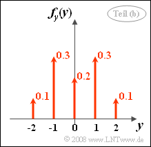
Discrete marginal PDF $f_{y}(y)$ 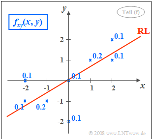
2D–PDF and regression line $\rm (RL)$
- The marginal probability density function $f_{x}(x)$ is obtained from the 2D–PDF $f_{xy}(x, y)$ by integration over $y$.
- For all possible values $ x \in \{-2, -1, \ 0, +1, +2\}$ the probabilities are equal $0.2$.
- It holds ${\rm Pr}(x \le 1)= 0.8$. The mean is $m_x = 0$.

(2) Correct are the proposed solutions 2 and 3:
- By integration over $x$ one obtains the PDF $f_{y}(y)$ sketched on the right.
- Due to symmetry, the mean value $m_y = 0$ is obtained.
- The probability we are looking for is ${\rm Pr}(y \le 1)= 0.9$.
(3) By definition:
- $$F_{xy}(r_x, r_y) = {\rm Pr} \big [(x \le r_x)\cap(y\le r_y)\big ].$$
- For $r_x = r_y = 1$ it follows:
- $$F_{xy}(+1, +1) = {\rm Pr}\big [(x \le 1)\cap(y\le 1)\big ].$$
- As can be seen from the 2D–PDF on the information page, this probability is ${\rm Pr}\big [(x \le 1)\cap(y\le 1)\big ]\hspace{0.15cm}\underline{=0.8}$.
(4) For this, Bayes' theorem can also be used to write:
- $$ \rm Pr(\it x \le \rm 1)\hspace{0.05cm} | \hspace{0.05cm} \it y \le \rm 1) = \frac{ \rm Pr\big [(\it x \le \rm 1)\cap(\it y\le \rm 1)\big ]}{ \rm Pr(\it y\le \rm 1)} = \it \frac{F_{xy} \rm (1, \rm 1)}{F_{y}\rm (1)}.$$
- With the results from (2) and (3) it follows $ \rm Pr(\it x \le \rm 1)\hspace{0.05cm} | \hspace{0.05cm} \it y \le \rm 1) = 0.8/0.9 = 8/9 \hspace{0.15cm}\underline{=0.889}$.
(5) According to the definition, the common moment is:
- $$m_{xy} = {\rm E}\big[x\cdot y \big] = \sum\limits_{i} {\rm Pr}( x_i \cap y_i)\cdot x_i\cdot y_i. $$
- There remain five Dirac delta functions with $x_i \cdot y_i \ne 0$:
- $$m_{xy} = \rm 0.1\cdot (-2) (-1) + 0.2\cdot(-1) (-1)+ 0.2\cdot 1\cdot 1 + 0.1\cdot 2\cdot 1+ 0.1\cdot 2\cdot 2\hspace{0.15cm}\underline{=\rm 1.2}.$$

(6) For the correlation coefficient:
- $$\rho_{xy} = \frac{\mu_{xy}}{\sigma_x\cdot \sigma_y} = \frac{1.2}{\sqrt{2}\cdot\sqrt{1.4}}\hspace{0.15cm}\underline{=0.717}.$$
- This takes into account that because $m_x = m_y = 0$ the covariance $\mu_{xy}$ is equal to the moment $m_{xy}$ .
- The equation of the correlation line is:
- $$y=\frac{\sigma_y}{\sigma_x}\cdot \rho_{xy}\cdot x = \frac{\mu_{xy}}{\sigma_x^{\rm 2}}\cdot x = \rm 0.6\cdot \it x.$$
- See sketch on the right. The angle between the regression line $\rm (RL)$ and the $x$-axis is
- $$\theta_{y\hspace{0.05cm}→\hspace{0.05cm} x} = \arctan(0.6) \hspace{0.15cm}\underline{=31^\circ}.$$
(7) The correct solutions are solutions 2 and 3:
- If statistically independent, $f_{xy}(x, y) = f_{x}(x) \cdot f_{y}(y)$ should hold, which is not done here.
- From correlatedness $($follows from $\rho_{xy} \ne 0)$ it is possible to directly infer statistical dependence,
- because correlation means a special form of statistical dependence, namely linear statistical dependence.