Exercise 4.3Z: Exponential and Laplace Distribution

Exponential PDF (above) d
Laplace PDF (below)

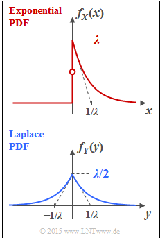
We consider here the probability density functions $\rm (PDF)$ of two continuous random variables:

The random variable $X$ is exponentially distributed (see top plot): For $x<0$ ⇒ $f_X(x) = 0$, and for positive $x$–values:

$$f_X(x) = \lambda \cdot {\rm e}^{-\lambda \hspace{0.05cm}\cdot \hspace{0.05cm}x}\hspace{0.05cm}. $$

On the other hand, for the Laplace distributed random variable $Y$ in the whole range $ - \infty < y < + \infty$ holds (lower sketch):

$$f_Y(y) = \lambda/2 \cdot {\rm e}^{-\lambda \hspace{0.05cm}\cdot \hspace{0.05cm}|\hspace{0.05cm}y\hspace{0.05cm}|}\hspace{0.05cm}.$$

To be calculated are the differential entropies $h(X)$ and $h(Y)$ depending on the PDF parameter $\it \lambda$. For example:

$$h(X) = -\hspace{-0.7cm} \int\limits_{x \hspace{0.05cm}\in \hspace{0.05cm}{\rm supp} \hspace{0.03cm}(\hspace{-0.03cm}f_X)} \hspace{-0.55cm} f_X(x) \cdot {\rm log} \hspace{0.1cm} \big [f_X(x) \big ] \hspace{0.1cm}{\rm d}x \hspace{0.05cm}.$$

If $\log_2$ is used, add the pseudo-unit "bit".

In subtasks (2) and (4) specify the differential entropy in the following form:

$$h(X) = {1}/{2} \cdot {\rm log} \hspace{0.1cm} ({\it \Gamma}_{{\hspace{-0.01cm} \rm L}}^{\hspace{0.08cm}(X)} \cdot \sigma^2), \hspace{0.8cm}h(Y) = {1}/{2} \cdot {\rm log} \hspace{0.1cm} ({\it \Gamma}_{{\hspace{-0.05cm} \rm L}}^{\hspace{0.08cm}(Y)} \cdot \sigma^2) \hspace{0.05cm}.$$

Determine by which factor ${\it \Gamma}_{{\hspace{-0.05cm} \rm L}}^{\hspace{0.08cm}(X)}$ the exponential PDF is characterized and which factor ${\it \Gamma}_{{\hspace{-0.01cm} \rm L}}^{\hspace{0.08cm}(Y)}$ results for the Laplace PDF.

Hints:

The exercise belongs to the chapter Differential Entropy.
Useful hints for solving this task can be found in particular on the page Differential entropy of some power-constrained random variables.
For the variance of the exponentially distributed random variable $X$ holds, as derived in Exercise 4.1Z: $\sigma^2 = 1/\lambda^2$.
The variance of the Laplace distributed random variable $Y$ is twice as large for the same $\it \lambda$: $\sigma^2 = 2/\lambda^2$.

Questions

$h(X) \ = \ $

$\ \rm bit$

${\it \Gamma}_{{\hspace{-0.01cm} \rm L}}^{\hspace{0.08cm}(X)} \ = \ $

$h(Y) \ = \ $

$\ \rm bit$

${\it \Gamma}_{{\hspace{-0.01cm} \rm L}}^{\hspace{0.08cm}(Y)} \ = \ $

Solution

(1) Although in this exercise the result should be given in "bit", we use the natural logarithm for derivation.

Then the differential entropy is:

$$h(X) = -\hspace{-0.7cm} \int\limits_{x \hspace{0.05cm}\in \hspace{0.05cm}{\rm supp} \hspace{0.03cm}(\hspace{-0.03cm}f_X)} \hspace{-0.35cm} f_X(x) \cdot {\rm ln} \hspace{0.1cm} \big [f_X(x)\big] \hspace{0.1cm}{\rm d}x \hspace{0.05cm}.$$

For the exponential distribution, the integration limits are $0$ and $+∞$. In this range, the PDF $f_X(x)$ according to the specification sheet is used:

$$h(X) =- \int_{0}^{\infty} \hspace{-0.15cm} \lambda \cdot {\rm e}^{-\lambda \hspace{0.05cm}\cdot \hspace{0.05cm}x} \hspace{0.05cm} \cdot \hspace{0.05cm} \left [ {\rm ln} \hspace{0.1cm} (\lambda) + {\rm ln} \hspace{0.1cm} ({\rm e}^{-\lambda \hspace{0.05cm}\cdot \hspace{0.05cm}x})\right ]\hspace{0.1cm}{\rm d}x - \hspace{0.05cm} {\rm ln} \hspace{0.1cm} (\lambda) \cdot \int_{0}^{\infty} \hspace{-0.15cm} \lambda \cdot {\rm e}^{-\lambda \hspace{0.05cm}\cdot \hspace{0.05cm}x}\hspace{0.1cm}{\rm d}x \hspace{0.1cm} + \hspace{0.1cm} \lambda \cdot \int_{0}^{\infty} \hspace{-0.15cm} \lambda \cdot x \cdot {\rm e}^{-\lambda \hspace{0.05cm}\cdot \hspace{0.05cm}x}\hspace{0.1cm}{\rm d}x \hspace{0.05cm}.$$

We can see:

The first integrand is identical to the PDF $f_X(x)$ considered here. Thus, the integral over the entire integration domain yields $1$.
The second integral corresponds exactly to the definition of the mean value $m_1$ (moment of first order). For the exponential PDF, $m_1 = 1/λ$ holds. From this follows:

$$h(X) = - \hspace{0.05cm} {\rm ln} \hspace{0.1cm} (\lambda) + 1 = - \hspace{0.05cm} {\rm ln} \hspace{0.1cm} (\lambda) + \hspace{0.05cm} {\rm ln} \hspace{0.1cm} ({\rm e}) = {\rm ln} \hspace{0.1cm} ({\rm e}/\lambda) \hspace{0.05cm}.$$

This result is to be given the additional unit "nat". Using $\log_2$ instead of $\ln$, we obtain the differential entropy in "bit":

$$h(X) = {\rm log}_2 \hspace{0.1cm} ({\rm e}/\lambda) \hspace{0.3cm} \Rightarrow \hspace{0.3cm} \lambda = 1{\rm :} \hspace{0.3cm} h(X) = {\rm log}_2 \hspace{0.1cm} ({\rm e}) = \frac{{\rm ln} \hspace{0.1cm} ({\rm e})}{{\rm ln} \hspace{0.1cm} (2)} \hspace{0.15cm}\underline{= 1.443\,{\rm bit}} \hspace{0.05cm}.$$

(2) Considering the equation $\sigma^2 = 1/\lambda^2$ valid for the exponential distribution, we can transform the result found in (1) as follows:

$$h(X) = {\rm log}_2 \hspace{0.1cm} ({\rm e}/\lambda) = {1}/{2}\cdot {\rm log}_2 \hspace{0.1cm} ({\rm e}^2/\lambda^2) = {1}/{2} \cdot {\rm log}_2 \hspace{0.1cm} ({\rm e}^2 \cdot \sigma^2) \hspace{0.05cm}.$$

A comparison with the required basic form $h(X) = {1}/{2} \cdot {\rm log}_2 \hspace{0.1cm} ({\it \Gamma}_{\hspace{-0.05cm} \rm L}^{\hspace{0.08cm}(X)} \cdot \sigma^2)$ leads to the result:

$${\it \Gamma}_{{\hspace{-0.05cm} \rm L}}^{\hspace{0.08cm}(X)} = {\rm e}^2 \hspace{0.15cm}\underline{\approx 7.39} \hspace{0.05cm}.$$

(3) For the Laplace distribution, we divide the integration domain into two subdomains:

$Y$ negative ⇒ proportion $h_{\rm neg}(Y)$,
$Y$ positive ⇒ proportion $h_{\rm pos}(Y)$.

The total differential entropy, taking into account $h_{\rm neg}(Y) = h_{\rm pos}(Y)$ is given by

$$h(Y) = h_{\rm neg}(Y) + h_{\rm pos}(Y) = 2 \cdot h_{\rm pos}(Y) $$

$$\Rightarrow \hspace{0.3cm} h(Y) = - 2 \cdot \int_{0}^{\infty} \hspace{-0.15cm} \lambda/2 \cdot {\rm e}^{-\lambda \hspace{0.05cm}\cdot \hspace{0.05cm}y} \hspace{0.05cm} \cdot \hspace{0.05cm} \left [ {\rm ln} \hspace{0.1cm} (\lambda/2) + {\rm ln} \hspace{0.1cm} ({\rm e}^{-\lambda \hspace{0.05cm}\cdot \hspace{0.05cm}y})\right ]\hspace{0.1cm}{\rm d}y = - \hspace{0.05cm} {\rm ln} \hspace{0.1cm} (\lambda/2) \cdot \int_{0}^{\infty} \hspace{-0.15cm} \lambda \cdot {\rm e}^{-\lambda \hspace{0.05cm}\cdot \hspace{0.05cm}y}\hspace{0.1cm}{\rm d}y \hspace{0.1cm} + \hspace{0.1cm} \lambda \cdot \int_{0}^{\infty} \hspace{-0.15cm} \lambda \cdot y \cdot {\rm e}^{-\lambda \hspace{0.05cm}\cdot \hspace{0.05cm}y}\hspace{0.1cm}{\rm d}y \hspace{0.05cm}.$$

If we again consider that the first integral gives the value $1$ (PDF area) and the second integral gives the mean value $m_1 = 1/\lambda$ we obtain:

$$h(Y) = - \hspace{0.05cm} {\rm ln} \hspace{0.1cm} (\lambda/2) + 1 = - \hspace{0.05cm} {\rm ln} \hspace{0.1cm} (\lambda/2) + \hspace{0.05cm} {\rm ln} \hspace{0.1cm} ({\rm e}) = {\rm ln} \hspace{0.1cm} (2{\rm e}/\lambda) \hspace{0.05cm}.$$

Since the result is required in "bit", we still need to replace "$\ln$" by "$\log_2$":

$$h(Y) = {\rm log}_2 \hspace{0.1cm} (2{\rm e}/\lambda) \hspace{0.3cm} \Rightarrow \hspace{0.3cm} \lambda = 1{\rm :} \hspace{0.3cm} h(Y) = {\rm log}_2 \hspace{0.1cm} (2{\rm e}) \hspace{0.15cm}\underline{= 2.443\,{\rm bit}} \hspace{0.05cm}.$$

(4) For the Laplace distribution, the relation $\sigma^2 = 2/\lambda^2$ holds. Thus, we obtain:

$$h(X) = {\rm log}_2 \hspace{0.1cm} (\frac{2{\rm e}}{\lambda}) = {1}/{2} \cdot {\rm log}_2 \hspace{0.1cm} (\frac{4{\rm e}^2}{\lambda^2}) = {1}/{2} \cdot {\rm log}_2 \hspace{0.1cm} (2 {\rm e}^2 \cdot \sigma^2) \hspace{0.3cm} \Rightarrow \hspace{0.3cm} {\it \Gamma}_{{\hspace{-0.05cm} \rm L}}^{\hspace{0.08cm}(Y)} = 2 \cdot {\rm e}^2 \hspace{0.15cm}\underline{\approx 14.78} \hspace{0.05cm}.$$

Consequently, the ${\it \Gamma}_{{\hspace{-0.05cm} \rm L}}$ value is twice as large for the Laplace distribution as for the exponential distribution.
Thus, the Laplace PDF is better than the exponential PDF in terms of differential entropy when power-limited signals are assumed.
Under the constraint of peak limitation, both the exponential and Laplace PDF are completely unsuitable, as is the Gaussian PDF. These all extend to infinity.