Exercise 4.4: Two-dimensional Gaussian PDF
From LNTwww
(Redirected from Exercise 4.4: Gaussian 2D PDF)

We consider two-dimensional random variables, where both components are always assumed to be mean-free.
- The »two-dimensional probability density function« of the random variable $(u, v)$ is:
- $$f_{uv}(u, v)={1}/{\pi} \cdot {\rm e}^{-(2u^{\rm 2} \hspace{0.05cm}+ \hspace{0.05cm}v^{\rm 2}\hspace{-0.05cm}/\rm 2)}.$$
- For another Gaussian two-dimensional random variable $(x, y)$ the following parameters are known:
- $$\sigma_x= 0.5, \hspace{0.5cm}\sigma_y = 1,\hspace{0.5cm}\rho_{xy} = 1. $$
- In the adjacent table can be found
- the values of the »Gaussian cumulative distribution function« ${\rm \phi}(x)$ and
- the »complementary function« ${\rm Q}(x) = 1- {\rm \phi}(x)$.
Hints:
- The exercise belongs to the chapter »Two-dimensional Gaussian Random Variables«.
- Reference is also made to the chapter »Gaussian distributed random variables«.
Questions
Solution
(1) Both statements are true:
$\rm Pr\big[(\it u < \rm 1) \cap (\it v > \rm 1)\big]$ 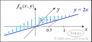
"Dirac wall" on the correlation line 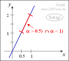
Probability calculation for the Dirac wall
- Comparing the given 2D–PDF with the general 2D–PDF
- $$f_{uv}(u,v) = \frac{\rm 1}{{\rm 2}\it\pi \cdot \sigma_u \cdot \sigma_v \cdot \sqrt{{\rm 1}-\it \rho_{\it uv}^{\rm 2}}} \cdot \rm exp\left[\frac{\rm 1}{2\cdot (\rm 1-\it \rho_{uv}^{\rm 2}{\rm )}}(\frac{\it u^{\rm 2}}{\it\sigma_u^{\rm 2}} + \frac{\it v^{\rm 2}}{\it\sigma_v^{\rm 2}} - \rm 2\it\rho_{uv}\frac{\it u\cdot \it v}{\sigma_u\cdot \sigma_v}\rm )\right],$$
- so it can be seen that no term with $u \cdot v$ occurs in the exponent, which is only possible with $\rho_{uv} = 0$.
- But this means that $u$ and $v$ are uncorrelated.
- For Gaussian random variables, however, statistical independence always follows from uncorrelatedness.
(2) With statistical independence holds:
- $$f_{uv}(u, v) = f_u(u)\cdot f_v(v) $$
- $$f_u(u)=\frac{{\rm e}^{-{\it u^{\rm 2}}/{(2\sigma_u^{\rm 2})}}}{\sqrt{\rm 2\pi}\cdot\sigma_u} , $$
- $$\it f_v{\rm (}v{\rm )}=\frac{{\rm e}^{-{\it v^{\rm 2}}/{{\rm (}{\rm 2}\sigma_v^{\rm 2}{\rm )}}}}{\sqrt{\rm 2\pi}\cdot\sigma_v}.$$
- By comparing coefficients, we get $\sigma_u = 0.5$ and $\sigma_v = 1$.
- The quotient is thus $\sigma_u/\sigma_v\hspace{0.15cm}\underline{=0.5}$.
(3) Because $u$ is a continuous random variable:
- $$\rm Pr(\it u < \rm 1) = \rm Pr(\it u \le \rm 1) =\it F_u\rm (1). $$
- With the mean $m_u = 0$ and the standard deviation $\sigma_u = 0.5$ we get:
- $$\rm Pr(\it u < \rm 1) = \rm \phi({\rm 1}/{\it\sigma_u})= \rm \phi(\rm 2) \hspace{0.15cm}\underline{=\rm 0.9772}. $$

(4) Due to the statistical independence between $u$ and $v$ holds:
- $$\rm Pr\big[(\it u < \rm 1) \cap (\it v > \rm 1)\big] = \rm Pr(\it u < \rm 1)\cdot \rm Pr(\it v > \rm 1).$$
- The probability ${\rm Pr}(u < 1) =0.9772$ has already been calculated.
- For the second probability ${\rm Pr}(v > 1)$ holds for reasons of symmetry:
- $$\rm Pr(\it v > \rm 1) = \rm Pr(\it v \le \rm (-1) = \it F_v\rm (-1) = \rm \phi(\frac{\rm -1}{\it\sigma_v}) = \rm Q(1) =0.1587$$
- $$\Rightarrow \hspace{0.3cm} \rm Pr\big[(\it u < \rm 1) \cap (\it v > \rm 1)\big] = \rm 0.9772\cdot \rm 0.1587 \hspace{0.15cm}\underline{ = \rm 0.1551}.$$
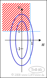
The sketch on the right illustrates the given constellation:
- The PDF contour lines (blue) are stretched ellipses due to $\sigma_v > \sigma_u$ in vertical direction.
- Drawn in red (shading) is the area whose probability should be calculated in this subtask.

(5) Correct are the first and the third suggested solutions:
- Because $\rho_{xy} = 1$ there is a deterministic correlation between $x$ and $y$
- ⇒ All values lie on the straight line $y =K \cdot x$.
- Because of the standard deviations $\sigma_x = 0.5$ and $\sigma_y = 1$ it holds $K = 2$.
- On this straight line $y = 2x$ ⇒ all PDF values are infinitely large.
- This means: The joint PDF is here a "Dirac wall".
- As you can see from the sketch, the PDF values are Gaussian distributed on the straight line $y = 2x$.
- The two marginal probability densities are also Gaussian functions, each with zero mean.
- Because of $\sigma_x = \sigma_u$ and $\sigma_y = \sigma_v$ also holds:
- $$f_x(x) = f_u(u), \hspace{0.5cm}f_y(y) = f_v(v).$$

(6) Since the PDF of the random variable $x$ is identical to the PDF $f_u(u)$, it also results in exactly the same probability as calculated in the subtask (3):
- $$\rm Pr(\it x < \rm 1) \hspace{0.15cm}\underline{ = \rm 0.9772}.$$
(7) The random event $y > 1$ is identical to the event $x > 0.5$.
- Thus, the wanted probability is equal to:
- $${\rm Pr}\big[(x < 1) ∩ (y > 1)\big] = \rm Pr \big[ (\it x < \rm 1)\cap (\it x > \rm 0.5) \big] = \it F_x \rm( 1) - \it F_x\rm (0.5). $$
- With the standard deviation $\sigma_x = 0.5$ it follows further:
- $$\rm Pr \big[(\it x > \rm 0.5) \cap (\it x < \rm 1)\big] = \rm \phi(\rm 2) - \phi(1)=\rm 0.9772- \rm 0.8413\hspace{0.15cm}\underline{=\rm 0.1359}.$$