Exercise 4.5: Two-dimensional Examination Evaluation
From LNTwww
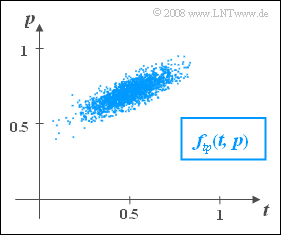
In a study, the master craftsman examinations were investigated, which always consist of a theoretical and additionally a practical part. In the graph denoted:
- $t$ is the score in the theoretical test,
- $p$ is the score in the practical test.
Both random variables $(t$ and $p)$ are normalized to the maximum and can therefore only take values between $0$ and $1$.
Moreover, both random variables are to be interpreted as continuous random variables, i.e.: $t$ and $p$ are not restricted to discrete numerical values.
- The graph shows the PDF $f_{tp}(t, p)$ of the two-dimensional random variable $(t,\hspace{0.08cm} p)$, which was published after evaluating a total of $N = 10\hspace{0.08cm}000$ final papers.
- This function was empirically approximated using an evaluation program as follows:
- $$f_{tp}(t,\hspace{0.08cm} p) = \rm 13.263\cdot \rm exp \Bigg\{-\frac{(\it t - \rm 0.5)^{\rm 2}}{\rm 0.0288}-\frac{(\it p-\rm 0.7)^{\rm 2}}{\rm 0.0072} + \frac{(\it t-\rm 0.5)(\it p-\rm 0.7)}{\rm 0.0090}\Bigg\}.$$
Hints:
- The exercise belongs to the chapter Two-dimensional Gaussian Random Variables.
- Reference is also made to the chapter Gaussian distributed random variables.
- More information on this topic is provided in the (German language) learning video "Gaußsche 2D-Zufallsgrößen":
- Part 1: Gaussian random variables without statistical bindings,
- Part 2: Gaussian random variables with statistical bindings.
Questions
Solution
(1) and (2)
- The mean values $m_t\hspace{0.15cm}\underline{= 0.5}$ and $m_p\hspace{0.15cm}\underline{= 0.7}$ can be estimated from the sketch and obtained exactly from the given equation.
- The 2D–PDF of the zero mean variable is:
- $$f_{\it t\hspace{0.05cm}'\hspace{0.05cm}p\hspace{0.05cm}'}(\it t\hspace{0.05cm}',\hspace{0.08cm} \it p\hspace{0.05cm}'{\rm )} = \rm 13.263\cdot \rm exp\Bigg (-\frac{\it {\rm (}t\hspace{0.05cm}'{\rm )}^{\rm 2}}{\rm 0.0288} - \frac{\it {\rm (}p\hspace{0.05cm}'{\rm )}^{\rm 2}}{\rm 0.0072}+\frac{\it t\hspace{0.05cm}'\cdot p\hspace{0.05cm}'}{\rm 0.0090}\Bigg ). $$
- For simplicity, the apostrophe is omitted below to denote zero mean variables.
- Both $t$ and $p$ are to be understood as zero mean up to and including the subtask (4).
(3) The general equation of a zero mean two-dimensional random variable is:
- $$f_{\it tp}(\it t,\hspace{0.08cm} \it p)=\frac{\rm 1}{\rm 2\it \pi \cdot \sigma_{\it t}\cdot \sigma_{\it p} \cdot\sqrt{\rm 1- \it\rho^{\rm 2}}}\hspace{0.1cm}\cdot \hspace{0.1cm}\rm exp\Bigg\{-\hspace{0.1cm}\frac{\it t^{\rm 2}}{\rm 2\cdot (\rm 1-\rho^{\rm 2})\cdot \sigma_{\it t}^{\rm 2}} -\hspace{0.1cm}\frac{\it p^{\rm 2}}{\rm 2\cdot (\rm 1-\it\rho^{\rm 2}{\rm )}\cdot \sigma_{\it p}^{\rm 2}}+\hspace{0.1cm}\frac{\rho\cdot \it t\cdot \it p}{ (\rm 1-\it \rho^{\rm 2}{\rm )}\cdot\sigma_{\it t}\cdot\sigma_{\it p}}\Bigg\}.$$
- The standard deviations $\sigma_t$ and $\sigma_p$ as well as the correlation coefficient $\rho$ can be obtained by coefficient comparison:
- A comparison of the first two terms in the exponent shows that $\sigma_t = 2 \cdot \sigma_p$ must hold. Thus the PDF is:
- $$f_{\it tp}(\it t,\hspace{0.08cm} \it p)=\frac{\rm 1}{\rm 4\it \pi \cdot \sigma_{\it p}^{\rm 2} \cdot\sqrt{\rm 1- \it\rho^{\rm 2}}}\hspace{0.1cm}\cdot \hspace{0.1cm}\rm exp\Bigg\{-\hspace{0.1cm}\frac{\it t^{\rm 2}}{\rm 8\cdot (\rm 1-\rho^{\rm 2})\cdot \sigma_{\it p}^{\rm 2}} -\hspace{0.1cm}\frac{\it p^{\rm 2}}{\rm 2\cdot (\rm 1-\it\rho^{\rm 2}{\rm )}\cdot \sigma_{\it p}^{\rm 2}}+\hspace{0.1cm}\frac{\rho\cdot \it t\cdot \it p}{\rm 2\cdot (\rm 1-\it \rho^{\rm 2}{\rm )}\cdot\sigma_{\it p}^{\rm 2}}\Bigg\}.$$
- From the second term of the exponent follows:
- $$2\cdot(1-\rho^{\rm 2})\cdot\sigma_{p}^{ 2}=0.0072\hspace{0.5cm}\Rightarrow \hspace{0.5cm} \sigma_{p}^{2} = \frac{ 0.0036}{(1-\rho^{\rm 2})}.$$
- The factor $K = 13.263$ now gives the result:
- $$K = \frac{\sqrt{\rm 1-\it\rho^{\rm 2}}}{\rm 4\it\pi\cdot \rm 0.0036}=\rm 13.263 \hspace{0.5cm}\Rightarrow \hspace{0.5cm}\sqrt{\rm 1-\it\rho^{\rm 2}}=\rm 0.6 \hspace{0.5cm}\Rightarrow \hspace{0.5cm}\hspace{0.15cm}\underline{ \rm \rho = \rm 0.8}.$$
- From this we get the standard deviations to $\sigma_t\hspace{0.15cm}\underline{= 0.2}$ and $\sigma_p\hspace{0.15cm}\underline{= 0.1}$.
- For control, we use the last term of the exponent:
- $$\frac{(1 - \rho^{2})\cdot \sigma_{\it t}\cdot\sigma_{\it p}}{\it \rho} = \frac{0.36\cdot 0.1\cdot 0.2}{0.8} = \rm 0.009.$$
- This agrees with the given value.
(4) The proposed solution 1 is correct.
- Basically, $(t,\hspace{0.08cm} p)$ is not a true Gaussian random variable, since both components are bounded.
- The probabilities for the events $t < 0$, $t >1$, $p < 0$ and $p >1$ are therefore zero.
- However, for Gaussian variables with the mean values and standard deviations present here, we get:
- $$\rm Pr(\it t < \rm 0) = \rm Pr(\it t > \rm 1) = \rm Q(2.5)\approx 6\cdot 10^{-3},$$
- $$\rm Pr(\it p > \rm 1) = \rm Q(3)\approx 1.3\cdot 10^{-3},$$
- $$\rm Pr(\it p < \rm 0) = \rm Q(7)\approx 10^{-12}.$$
- The correlation coefficient $\rho = 0.8$ is positive here. If the examinee has done rather well in the theory part, it is to be expected (at least for this exercise) that the practical part will also go well.
- Suggestion 2 is therefore wrong. In practice, this is certainly not always the case.
(5) For this probability with $\Delta t = \Delta p = 0.02$:
- $$\rm Pr\left [( \rm 0.5-\frac{\rm\Delta\it t}{\rm 2}\le \it t \le \rm 0.5+\frac{\rm\Delta\it t}{\rm 2})\cap(\rm 0. 5-\frac{\rm\Delta\it p}{\rm 2}\le \it p \le \rm 0.5+\frac{\rm\Delta\it p}{\rm 2})\right ] \approx \rm\Delta\it t\cdot\rm\Delta\it p\cdot \it f_{tp}{\rm (}t=\rm 0.5, \it p = \rm 0.5).$$
- For the 2D–PDF, taking into account the mean values $m_t{= 0.5}$ and $m_p{= 0.7}$:
- $$f_{tp}(\it t=\rm 0.5,\hspace{0.08cm} \it p=\rm 0.5) = \rm 13.263\cdot {\rm e}^{-(-0.2)^2/0.0072}\approx 0.0513.$$
- Thus, the probability we are looking for is given by
- $${\rm Pr}\big[(0.49 ≤ t ≤0.51)∩(0.49≤ p ≤0.51)\big] =0.02 \cdot 0.0513\hspace{0.15cm}\underline{\approx 2 · 10^{-5}}.$$
