Difference between revisions of "Aufgaben:Exercise 2.2Z: Non-Linearities"
From LNTwww
m (Oezdemir moved page Aufgabe 2.2Z: Nichtlinearitäten to Exercise 2.2Z: Nonlinearities) |
|||
| Line 4: | Line 4: | ||
[[File:P_ID322__Sig_Z_2_2.png|right|frame|Gleichanteil nach Nichtlinearitäten]] | [[File:P_ID322__Sig_Z_2_2.png|right|frame|Gleichanteil nach Nichtlinearitäten]] | ||
| − | + | We start from the triangular signal ${x(t)}$ according to the figure above. | |
| − | + | If we apply this signal to an amplitude limiter, we get the signal | |
:$$y(t)=\left\{ {x(t)\atop \rm 1V}{\hspace{0.5cm} {\rm f\ddot{u}r}\quad x(t)\le \rm 1V \atop {\rm sonst}}\right..$$ | :$$y(t)=\left\{ {x(t)\atop \rm 1V}{\hspace{0.5cm} {\rm f\ddot{u}r}\quad x(t)\le \rm 1V \atop {\rm sonst}}\right..$$ | ||
| − | + | A second non-linearity provides the signal | |
:$$z(t)=x^2(t).$$ | :$$z(t)=x^2(t).$$ | ||
| − | + | The DC signal components are designated $x_0$, $y_0$ and $z_0$ in the following. | |
| Line 19: | Line 19: | ||
| − | '' | + | ''Hint:'' |
| − | * | + | *This exercise belongs to the chapter [[Signal_Representation/Direct_Current_Signal_-_Limit_Case_of_a_Periodic_Signal|Direct Current Signal - Limit Case of a Periodic Signal.]]. |
| Line 27: | Line 27: | ||
| − | === | + | ===Questions=== |
<quiz display=simple> | <quiz display=simple> | ||
| − | { | + | {Determine the DC signal component $x_0$ of the signal ${x(t)}$. |
|type="{}"} | |type="{}"} | ||
$x_0\ = \ $ { 1 3% } $\text{V}$ | $x_0\ = \ $ { 1 3% } $\text{V}$ | ||
| − | { | + | {Determine the DC signal component $y_0$ of the signal ${y(t)}$. |
|type="{}"} | |type="{}"} | ||
$y_0\ = \ $ { 0.75 3% } $\text{V}$ | $y_0\ = \ $ { 0.75 3% } $\text{V}$ | ||
| − | { | + | {Determine the DC signal component $z_0$ of the signal ${z(t)}$. |
|type="{}"} | |type="{}"} | ||
$z_0\ = \ $ { 1.333 3% } $\text{V}^2$ | $z_0\ = \ $ { 1.333 3% } $\text{V}^2$ | ||
| Line 48: | Line 48: | ||
</quiz> | </quiz> | ||
| − | === | + | ===Solution=== |
{{ML-Kopf}} | {{ML-Kopf}} | ||
| − | '''(1)''' | + | '''(1)''' The DC signal $x_0$ is the mean value of the signal ${x(t)}$. Averaging over a period duration $T_0 = 1 \, \text{ms}$ is sufficient. One obtains: |
:$$x_0=\frac{1}{T_0}\int^{T_0}_0 x(t)\,{\rm d} t \hspace{0.15cm}\underline{=1\,\rm V}.$$ | :$$x_0=\frac{1}{T_0}\int^{T_0}_0 x(t)\,{\rm d} t \hspace{0.15cm}\underline{=1\,\rm V}.$$ | ||
| − | '''(2)''' In | + | '''(2)''' In half the time ${y(t)} = 1\, \text{V}$, in the other half is is between $0$ and $1\, \text{V}$ with the mean value at $0.5 \,\text{V}$ ⇒ $y_0 \hspace{0.15cm}\underline{= 0.75 \,\text{V}}$. |
| − | '''(3)''' | + | '''(3)''' Due to the periodicity and symmetry, averaging in the range from $0$ bis $T_0/2$ is sufficient. |
| − | * | + | * With the corresponding characteristic curve, the following then applies:: |
:$$z_0=\frac{1}{T_0/2}\int^{T_0/2}_0 x^2(t)\,{\rm d}t=\frac{4\rm V^2}{T_0/2}\int^{T_0/2}_0 ({2t}/{T_0})^2\, {\rm d}t={4}/{3}\rm \;V^2 | :$$z_0=\frac{1}{T_0/2}\int^{T_0/2}_0 x^2(t)\,{\rm d}t=\frac{4\rm V^2}{T_0/2}\int^{T_0/2}_0 ({2t}/{T_0})^2\, {\rm d}t={4}/{3}\rm \;V^2 | ||
\hspace{0.15cm}\underline{\approx1.333\rm \;V^2}.$$ | \hspace{0.15cm}\underline{\approx1.333\rm \;V^2}.$$ | ||
Revision as of 03:14, 4 January 2021
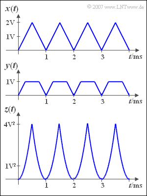
We start from the triangular signal ${x(t)}$ according to the figure above.
If we apply this signal to an amplitude limiter, we get the signal
- $$y(t)=\left\{ {x(t)\atop \rm 1V}{\hspace{0.5cm} {\rm f\ddot{u}r}\quad x(t)\le \rm 1V \atop {\rm sonst}}\right..$$
A second non-linearity provides the signal
- $$z(t)=x^2(t).$$
The DC signal components are designated $x_0$, $y_0$ and $z_0$ in the following.
Hint:
- This exercise belongs to the chapter Direct Current Signal - Limit Case of a Periodic Signal..
Questions
Solution
(1) The DC signal $x_0$ is the mean value of the signal ${x(t)}$. Averaging over a period duration $T_0 = 1 \, \text{ms}$ is sufficient. One obtains:
- $$x_0=\frac{1}{T_0}\int^{T_0}_0 x(t)\,{\rm d} t \hspace{0.15cm}\underline{=1\,\rm V}.$$
(2) In half the time ${y(t)} = 1\, \text{V}$, in the other half is is between $0$ and $1\, \text{V}$ with the mean value at $0.5 \,\text{V}$ ⇒ $y_0 \hspace{0.15cm}\underline{= 0.75 \,\text{V}}$.
(3) Due to the periodicity and symmetry, averaging in the range from $0$ bis $T_0/2$ is sufficient.
- With the corresponding characteristic curve, the following then applies::
- $$z_0=\frac{1}{T_0/2}\int^{T_0/2}_0 x^2(t)\,{\rm d}t=\frac{4\rm V^2}{T_0/2}\int^{T_0/2}_0 ({2t}/{T_0})^2\, {\rm d}t={4}/{3}\rm \;V^2 \hspace{0.15cm}\underline{\approx1.333\rm \;V^2}.$$
