Difference between revisions of "Aufgaben:Exercise 3.8: Triple Convolution?"
| (4 intermediate revisions by 2 users not shown) | |||
| Line 7: | Line 7: | ||
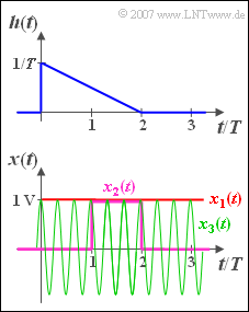
:$$h( t ) = \frac{1}{T}\cdot \left( {1 - \frac{t}{ {2T}}} \right).$$ | :$$h( t ) = \frac{1}{T}\cdot \left( {1 - \frac{t}{ {2T}}} \right).$$ | ||
| − | Outside this interval, $h(t) = 0$. The corresponding spectral function is: | + | Outside this interval, $h(t) = 0$. The corresponding spectral function is: |
:$$H( f ) = \frac{1}{ {8\left( {{\rm{\pi }}fT} \right)^2 }} \cdot \left( {1 - {\rm{j \cdot 4\pi }}fT - {\rm{e}}^{ - {\rm{j \hspace{0.05cm}\cdot \hspace{0.05cm} 4\pi }}\hspace{0.05cm}f\hspace{0.05cm}T} } \right).$$ | :$$H( f ) = \frac{1}{ {8\left( {{\rm{\pi }}fT} \right)^2 }} \cdot \left( {1 - {\rm{j \cdot 4\pi }}fT - {\rm{e}}^{ - {\rm{j \hspace{0.05cm}\cdot \hspace{0.05cm} 4\pi }}\hspace{0.05cm}f\hspace{0.05cm}T} } \right).$$ | ||
| − | This equation is not suitable for calculating the so-called & | + | This equation is not suitable for calculating the so-called "direct signal transfer factor" ⇒ $H(f = 0)$, since both the bracket expression and the denominator become zero. However, it is also valid: |
:$$H( {f = 0} ) = \int_0^{2T} {h( t )\hspace{0.1cm}{\rm d}t = 1.}$$ | :$$H( {f = 0} ) = \int_0^{2T} {h( t )\hspace{0.1cm}{\rm d}t = 1.}$$ | ||
| Line 17: | Line 17: | ||
Three different time signals are applied to the input of this filter (see sketch): | Three different time signals are applied to the input of this filter (see sketch): | ||
* $x_1(t)$ is a DC signal with height $x_0 = 1 \hspace{0.05cm}{\rm V}$. | * $x_1(t)$ is a DC signal with height $x_0 = 1 \hspace{0.05cm}{\rm V}$. | ||
| − | * $x_2(t)$ is a | + | * $x_2(t)$ is a rectangular pulse with duration $T$ and height $x_0 = 1\hspace{0.05cm} {\rm V}$, starting at $t = T$. |
* $x_3(t)$ is a cosine signal with frequency $f_0 = 3/T$ and amplitude $x_0 = 1 \hspace{0.05cm}{\rm V}$. | * $x_3(t)$ is a cosine signal with frequency $f_0 = 3/T$ and amplitude $x_0 = 1 \hspace{0.05cm}{\rm V}$. | ||
| Line 29: | Line 29: | ||
''Hints:'' | ''Hints:'' | ||
*This exercise belongs to the chapter [[Signal_Representation/The_Convolution_Theorem_and_Operation|The Convolution Theorem and Operation]]. | *This exercise belongs to the chapter [[Signal_Representation/The_Convolution_Theorem_and_Operation|The Convolution Theorem and Operation]]. | ||
| − | *The topic of this section is also illustrated in the [[Applets: | + | *The topic of this section is also illustrated in the interactive applet [[Applets:Graphical_Convolution| Graphical Convolution]]. |
| Line 42: | Line 42: | ||
- $y_3(t) = x_3(t) \ast h(t)$. | - $y_3(t) = x_3(t) \ast h(t)$. | ||
| − | {What is the signal $y_1(t)$ at the filter output when the DC signal $x_1(t) = 1 \hspace{0.03cm}{\rm V}$ is applied to the input? Give the signal value at $t = 2T$ | + | {What is the signal $y_1(t)$ at the filter output when the DC signal $x_1(t) = 1 \hspace{0.03cm}{\rm V}$ is applied to the input? Give the signal value at $t = 2T$. |
|type="{}"} | |type="{}"} | ||
$y_1(t=2T)\ = \ $ { 1 3% } ${\rm V}$ | $y_1(t=2T)\ = \ $ { 1 3% } ${\rm V}$ | ||
| Line 56: | Line 56: | ||
$y_2(t=3T)\ = \ $ { 0.25 3% } ${\rm V}$ | $y_2(t=3T)\ = \ $ { 0.25 3% } ${\rm V}$ | ||
| − | {What is the output signal $y_3(t)$, when the cosine signal $x_3(t)$ is applied to the input? Give the signal value at $t =0$ | + | {What is the output signal $y_3(t)$, when the cosine signal $x_3(t)$ is applied to the input? Give the signal value at $t =0$. |
|type="{}"} | |type="{}"} | ||
$y_3(t=0)\ = \ $ { 0. } ${\rm V}$ | $y_3(t=0)\ = \ $ { 0. } ${\rm V}$ | ||
| Line 66: | Line 66: | ||
{{ML-Kopf}} | {{ML-Kopf}} | ||
'''(1)''' The correct <u>answer is 2</u>: | '''(1)''' The correct <u>answer is 2</u>: | ||
| − | *$x_1(t)$ and $x_3(t)$ | + | *Both $x_1(t)$ and $x_3(t)$ contain only one frequency, namely $f = 0$ or $f = f_0$. In each case, the diversions via the spectrum is preferable. |
| − | * | + | *With the rectangular pulse $x_2(t)$ the calculation via convolution is more favourable, since the inverse Fourier transform of $Y_2(f)$ is complicated. |
| − | '''(2)''' For the | + | '''(2)''' For the signal $x_1(t)$ the output signal is also a DC signal, since the following equations apply: |
| − | :$$Y_1 (f) = X_1 (f) \cdot H(f)\quad {\rm{ | + | :$$Y_1 (f) = X_1 (f) \cdot H(f)\quad {\rm{with}}\quad X_1 (f) = 1\;{\rm{V}} \cdot \delta (f)$$ |
:$$ \Rightarrow Y_1 (f) = 1\;{\rm{V}} \cdot \delta (f) \cdot H( {f = 0} ) = 1\;{\rm{V}} \cdot \delta (f) \; \Rightarrow \; y_1 (t) = 1\;{\rm{V}} \cdot H( {f = 0} ) \hspace{0.15 cm}\underline{= 1\;{\rm{V}}}.$$ | :$$ \Rightarrow Y_1 (f) = 1\;{\rm{V}} \cdot \delta (f) \cdot H( {f = 0} ) = 1\;{\rm{V}} \cdot \delta (f) \; \Rightarrow \; y_1 (t) = 1\;{\rm{V}} \cdot H( {f = 0} ) \hspace{0.15 cm}\underline{= 1\;{\rm{V}}}.$$ | ||
| Line 80: | Line 80: | ||
'''(3)''' The mirrored signal $x_2(-t)$ has signal components between $-2T$ and $-T$. | '''(3)''' The mirrored signal $x_2(-t)$ has signal components between $-2T$ and $-T$. | ||
| − | *Only a shift by $T \hspace{-0.1cm}+ \hspace{-0.1cm}\varepsilon$ leads to an overlap with $h(t)$. Here $\varepsilon$ denotes an arbitrarily small but positive time. | + | *Only a shift by $T \hspace{-0.1cm}+ \hspace{-0.1cm}\varepsilon$ leads to an overlap with $h(t)$. Here $\varepsilon$ denotes an arbitrarily small but positive time. |
| − | *However, if the shift is greater than $4T\hspace{-0.1cm} - \hspace{-0.1cm}\varepsilon$, the integration over the product also yields the value zero. From this follows: | + | *However, if the shift is greater than $4T\hspace{-0.1cm} - \hspace{-0.1cm}\varepsilon$, the integration over the product also yields the value zero. From this follows: |
:$$t_{\text{min}} \;\underline{= T}, \ \ \ t_{\text{max}} \;\underline{= 4T}.$$ | :$$t_{\text{min}} \;\underline{= T}, \ \ \ t_{\text{max}} \;\underline{= 4T}.$$ | ||
| − | [[File:P_ID534__Sig_A_3_8_d.png|right|frame| | + | [[File:P_ID534__Sig_A_3_8_d.png|right|frame|"Rectangle" $\star$ "Triangle" ]] |
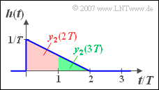
'''(4)''' The result of the graphical convolution for the times $t = 2T$ and $t = 3T$ can be seen in the adjacent sketch. | '''(4)''' The result of the graphical convolution for the times $t = 2T$ and $t = 3T$ can be seen in the adjacent sketch. | ||
*The value at $t = 2T$ corresponds to the area highlighted in red: | *The value at $t = 2T$ corresponds to the area highlighted in red: | ||
| Line 99: | Line 99: | ||
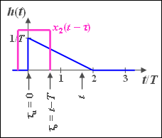
| + | '''(4a)''' For $T \leq t \leq 2T$ the lower $($German: "untere" ⇒ "u"$)$ limit is $τ_u = 0$, and the upper $($German: "obere" ⇒ "o"$)$ limit is $τ_0 = t - T$: | ||
[[File:P_ID583__Sig_A_3_8_d1_neu.png|right|frame|Convolution for $T \leq t \leq 2T$]] | [[File:P_ID583__Sig_A_3_8_d1_neu.png|right|frame|Convolution for $T \leq t \leq 2T$]] | ||
| − | |||
:$$y_2 (t) = \int_{\tau _u }^{\tau _0 } {h(\tau )\,{\rm{d}}\tau = \int_0^{t - T} {\frac{1}{T}} }\cdot \left( {1 - \frac{\tau }{ {2T}}} \right)\,{\rm{d}}\tau .$$ | :$$y_2 (t) = \int_{\tau _u }^{\tau _0 } {h(\tau )\,{\rm{d}}\tau = \int_0^{t - T} {\frac{1}{T}} }\cdot \left( {1 - \frac{\tau }{ {2T}}} \right)\,{\rm{d}}\tau .$$ | ||
| Line 109: | Line 109: | ||
:$$\Rightarrow \hspace{0.3cm}y_2 (t) = 1.5 \cdot {t}/{T} - 0.25\cdot \left( {{t}/{T}} \right)^2 - 1.25.$$ | :$$\Rightarrow \hspace{0.3cm}y_2 (t) = 1.5 \cdot {t}/{T} - 0.25\cdot \left( {{t}/{T}} \right)^2 - 1.25.$$ | ||
| − | *For verification we consider the two limits. We get the values $y_2(T) = 0$ and $y_2(2T) = 0.75$. | + | *For verification we consider the two limits. We get the values $y_2(T) = 0$ and $y_2(2T) = 0.75$. |
| − | + | <br clear=all> | |
| − | |||
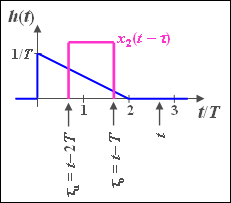
[[File:P_ID584__Sig_A_3_8_d2_neu.png|right|frame|Convolution for $2T \leq t \leq 3T$]] | [[File:P_ID584__Sig_A_3_8_d2_neu.png|right|frame|Convolution for $2T \leq t \leq 3T$]] | ||
| − | '''(4b)''' In the interval $2T \leq t \leq 3T$ | + | '''(4b)''' In the interval $2T \leq t \leq 3T$, the lower limit $τ_0 = t - T$ still holds, while now $τ_u = t - 2T$: |
::$$y_2 (t) = I(t - T) - I(t - 2T) = 1.75 - 0.5 \cdot {t}/{T}.$$ | ::$$y_2 (t) = I(t - T) - I(t - 2T) = 1.75 - 0.5 \cdot {t}/{T}.$$ | ||
| − | This corresponds to a linear decrease with the two limit values | + | This corresponds to a linear decrease with the two limit values: |
:$$y_2(2T) = 0.75,$$ | :$$y_2(2T) = 0.75,$$ | ||
:$$y_2(3T) = 0.25.$$ | :$$y_2(3T) = 0.25.$$ | ||
| Line 131: | Line 130: | ||
<br clear=all> | <br clear=all> | ||
'''(5)''' In principle, this sub-task could also be solved directly with the convolution. | '''(5)''' In principle, this sub-task could also be solved directly with the convolution. | ||
| − | *However, since $x_3(t)$ is an even function, the | + | *However, since $x_3(t)$ is an even function, the mirror can now be dispensed and we obtain: |
:$$y_3 (t) = \int_{ - \infty }^{ + \infty } {h(\tau ) \cdot x_3 (t + \tau )\hspace{0.1cm}{\rm{d}}\tau = x_0 }\cdot \int_0^{2T} {h(\tau ) \cdot \cos (2{\rm{\pi }}f_0 (t + \tau )\hspace{0.1cm}{\rm{d}}\tau .}$$ | :$$y_3 (t) = \int_{ - \infty }^{ + \infty } {h(\tau ) \cdot x_3 (t + \tau )\hspace{0.1cm}{\rm{d}}\tau = x_0 }\cdot \int_0^{2T} {h(\tau ) \cdot \cos (2{\rm{\pi }}f_0 (t + \tau )\hspace{0.1cm}{\rm{d}}\tau .}$$ | ||
| − | *The simpler way here is via the spectra. $X(f)$ consists of two diraclines at $\pm 3f_0$. Thus, the frequency response must also only be calculated for this frequency: | + | *The simpler way here is via the spectra. $X(f)$ consists of two diraclines at $\pm 3f_0$. Thus, the frequency response must also only be calculated for this frequency: |
:$$H( {f = 3f_0 } ) = \frac{1}{ {72{\rm{\pi }}^{\rm{2}} }}\big[ {1 - {\rm{j}}\cdot 12{\rm{\pi }} - {\rm{cos}}( {{\rm{12\pi }}} ) + {\rm{j}}\cdot \sin ( {{\rm{12\pi }}})} \big] = \frac{1}{ {72{\rm{\pi }}^{\rm{2}} }}\big[ 1 - {\rm j}\cdot 12{\rm \pi } - 1 + {\rm j}\cdot 0 \big]= { - {\rm{j}}} \cdot \frac{1}{ {6{\rm{\pi }}}}.$$ | :$$H( {f = 3f_0 } ) = \frac{1}{ {72{\rm{\pi }}^{\rm{2}} }}\big[ {1 - {\rm{j}}\cdot 12{\rm{\pi }} - {\rm{cos}}( {{\rm{12\pi }}} ) + {\rm{j}}\cdot \sin ( {{\rm{12\pi }}})} \big] = \frac{1}{ {72{\rm{\pi }}^{\rm{2}} }}\big[ 1 - {\rm j}\cdot 12{\rm \pi } - 1 + {\rm j}\cdot 0 \big]= { - {\rm{j}}} \cdot \frac{1}{ {6{\rm{\pi }}}}.$$ | ||
| Line 148: | Line 147: | ||
__NOEDITSECTION__ | __NOEDITSECTION__ | ||
| − | [[Category: | + | [[Category:Signal Representation: Exercises|^3.4 The Convolution Theorem^]] |
Latest revision as of 13:27, 29 April 2021
The impulse response of an LTI system has the following course in the time range between $0$ and $2T$ :
- $$h( t ) = \frac{1}{T}\cdot \left( {1 - \frac{t}{ {2T}}} \right).$$
Outside this interval, $h(t) = 0$. The corresponding spectral function is:
- $$H( f ) = \frac{1}{ {8\left( {{\rm{\pi }}fT} \right)^2 }} \cdot \left( {1 - {\rm{j \cdot 4\pi }}fT - {\rm{e}}^{ - {\rm{j \hspace{0.05cm}\cdot \hspace{0.05cm} 4\pi }}\hspace{0.05cm}f\hspace{0.05cm}T} } \right).$$
This equation is not suitable for calculating the so-called "direct signal transfer factor" ⇒ $H(f = 0)$, since both the bracket expression and the denominator become zero. However, it is also valid:
- $$H( {f = 0} ) = \int_0^{2T} {h( t )\hspace{0.1cm}{\rm d}t = 1.}$$
Three different time signals are applied to the input of this filter (see sketch):
- $x_1(t)$ is a DC signal with height $x_0 = 1 \hspace{0.05cm}{\rm V}$.
- $x_2(t)$ is a rectangular pulse with duration $T$ and height $x_0 = 1\hspace{0.05cm} {\rm V}$, starting at $t = T$.
- $x_3(t)$ is a cosine signal with frequency $f_0 = 3/T$ and amplitude $x_0 = 1 \hspace{0.05cm}{\rm V}$.
Hints:
- This exercise belongs to the chapter The Convolution Theorem and Operation.
- The topic of this section is also illustrated in the interactive applet Graphical Convolution.
Question
Solution
- Both $x_1(t)$ and $x_3(t)$ contain only one frequency, namely $f = 0$ or $f = f_0$. In each case, the diversions via the spectrum is preferable.
- With the rectangular pulse $x_2(t)$ the calculation via convolution is more favourable, since the inverse Fourier transform of $Y_2(f)$ is complicated.
(2) For the signal $x_1(t)$ the output signal is also a DC signal, since the following equations apply:
- $$Y_1 (f) = X_1 (f) \cdot H(f)\quad {\rm{with}}\quad X_1 (f) = 1\;{\rm{V}} \cdot \delta (f)$$
- $$ \Rightarrow Y_1 (f) = 1\;{\rm{V}} \cdot \delta (f) \cdot H( {f = 0} ) = 1\;{\rm{V}} \cdot \delta (f) \; \Rightarrow \; y_1 (t) = 1\;{\rm{V}} \cdot H( {f = 0} ) \hspace{0.15 cm}\underline{= 1\;{\rm{V}}}.$$
- The calculation via convolution leads to the same result if one takes into account that the integral over the impulse response is equal to $1$ in the present case.
(3) The mirrored signal $x_2(-t)$ has signal components between $-2T$ and $-T$.
- Only a shift by $T \hspace{-0.1cm}+ \hspace{-0.1cm}\varepsilon$ leads to an overlap with $h(t)$. Here $\varepsilon$ denotes an arbitrarily small but positive time.
- However, if the shift is greater than $4T\hspace{-0.1cm} - \hspace{-0.1cm}\varepsilon$, the integration over the product also yields the value zero. From this follows:
- $$t_{\text{min}} \;\underline{= T}, \ \ \ t_{\text{max}} \;\underline{= 4T}.$$
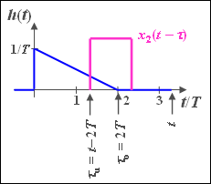
(4) The result of the graphical convolution for the times $t = 2T$ and $t = 3T$ can be seen in the adjacent sketch.
- The value at $t = 2T$ corresponds to the area highlighted in red:
- $$y_2( {t = 2T} ) = \frac{1}{2}\cdot ( {\frac{1}{T} + \frac{1}{ {2T}}} ) \cdot T \cdot x_0 \hspace{0.15 cm}\underline{= 0.75 {\rm V}} .$$
- The green highlighted area indicates the value at $t = 3T$:
- $$y_2( {t = 3T} ) = \frac{1}{2}\cdot ( {\frac{1}{2T} + 0} ) \cdot T \cdot x_0 \hspace{0.15 cm}\underline{= 0.25 {\rm V}} .$$
To calculate the entire signal curve between $t = T$ and $t = 4T$ three areas must be considered separately. To simplify the representation, $x_0 = 1$ is set in the following ⇒ amplitude normalisation.
(4a) For $T \leq t \leq 2T$ the lower $($German: "untere" ⇒ "u"$)$ limit is $τ_u = 0$, and the upper $($German: "obere" ⇒ "o"$)$ limit is $τ_0 = t - T$:
- $$y_2 (t) = \int_{\tau _u }^{\tau _0 } {h(\tau )\,{\rm{d}}\tau = \int_0^{t - T} {\frac{1}{T}} }\cdot \left( {1 - \frac{\tau }{ {2T}}} \right)\,{\rm{d}}\tau .$$
- With the indefinite integral $I(\tau ) = {\tau }/{T} - 0.25 \cdot \left( {{\tau }/{T}} \right)^2$ we obtain
- $$y_2 (t) = I(t - T) - I(0) = \frac{ {t - T}}{T} - 0.25 \cdot \left( {\frac{ {t - T}}{T}} \right)^2 $$
- $$\Rightarrow \hspace{0.3cm}y_2 (t) = 1.5 \cdot {t}/{T} - 0.25\cdot \left( {{t}/{T}} \right)^2 - 1.25.$$
- For verification we consider the two limits. We get the values $y_2(T) = 0$ and $y_2(2T) = 0.75$.
(4b) In the interval $2T \leq t \leq 3T$, the lower limit $τ_0 = t - T$ still holds, while now $τ_u = t - 2T$:
- $$y_2 (t) = I(t - T) - I(t - 2T) = 1.75 - 0.5 \cdot {t}/{T}.$$
This corresponds to a linear decrease with the two limit values:
- $$y_2(2T) = 0.75,$$
- $$y_2(3T) = 0.25.$$
(4c) For the interval $3T \leq t \leq 4T$ and $τ_0 = 2T$ und $τ_u = t - 2T$:
- $$y_2 (t) = I(2T) - I(t - 2T) = - 2 \cdot {t}/{T} + 0.25\left( {c{t}/{T}} \right)^2 + 4.$$
Here, too, the correct limit values result:
- $$y_2 (3T) = 0.25,$$
- $$y_2 (4T) = 0.$$
(5) In principle, this sub-task could also be solved directly with the convolution.
- However, since $x_3(t)$ is an even function, the mirror can now be dispensed and we obtain:
- $$y_3 (t) = \int_{ - \infty }^{ + \infty } {h(\tau ) \cdot x_3 (t + \tau )\hspace{0.1cm}{\rm{d}}\tau = x_0 }\cdot \int_0^{2T} {h(\tau ) \cdot \cos (2{\rm{\pi }}f_0 (t + \tau )\hspace{0.1cm}{\rm{d}}\tau .}$$
- The simpler way here is via the spectra. $X(f)$ consists of two diraclines at $\pm 3f_0$. Thus, the frequency response must also only be calculated for this frequency:
- $$H( {f = 3f_0 } ) = \frac{1}{ {72{\rm{\pi }}^{\rm{2}} }}\big[ {1 - {\rm{j}}\cdot 12{\rm{\pi }} - {\rm{cos}}( {{\rm{12\pi }}} ) + {\rm{j}}\cdot \sin ( {{\rm{12\pi }}})} \big] = \frac{1}{ {72{\rm{\pi }}^{\rm{2}} }}\big[ 1 - {\rm j}\cdot 12{\rm \pi } - 1 + {\rm j}\cdot 0 \big]= { - {\rm{j}}} \cdot \frac{1}{ {6{\rm{\pi }}}}.$$
- Thus the spectrum of the output signal is:
- $$Y(f) = - {\rm{j}} \cdot \frac{ {x_0 }}{{{\rm{12\pi }}}}\cdot \delta \left( {f - 3f_0 } \right) + {\rm{j}} \cdot \frac{ {x_0 }}{{{\rm{12\pi }}}}\cdot \delta \left( {f + 3f_0 } \right).$$
- The signal $y_3(t)$ is thus sinusoidal with amplitude $x_0/(6\pi )$.
- At $t = 0$ the signal value $y_3(t = 0)\; \underline{= 0}$ results.
