Difference between revisions of "Aufgaben:Exercise 3.8Z: Convolution of Two Rectangles"
m (Guenter moved page Exercise 3.8Z:Convolution of Two Rectangles to Exercise 3.8Z: Convolution of Two Rectangles) |
|||
| (5 intermediate revisions by 2 users not shown) | |||
| Line 3: | Line 3: | ||
}} | }} | ||
| − | [[File:P_ID535__Sig_Z_3_8.png|right|frame| | + | [[File:P_ID535__Sig_Z_3_8.png|right|frame|The convolution of two rectangles $x(t)$ and $h(t)$ |
]] | ]] | ||
| − | At the input of a causal LTI system (i.e. linear and time-invariant) with a rectangular impulse response ${h(t)}$ of duration $2 \,\text{ms}$ , a rectangular | + | At the input of a causal LTI system (i.e. linear and time-invariant) |
| + | *with a rectangular impulse response ${h(t)}$ of duration $2 \,\text{ms}$ , | ||
| + | *a rectangular pulse ${x(t)}$ of duration $T = 3 \,\text{ms}$ and amplitude $A = 2\,\text{ V}$ is applied. | ||
| − | |||
| − | |||
| − | |||
| + | The rectangular functions each start at the time $t = 0$. | ||
| + | |||
| + | In this task you are to calculate the output signal ${y(t)}$ with the help of the "Graphical Convolution". | ||
| + | As you can easily check, the output signal ${y(t)}$ | ||
| + | *differs from zero only in the range between $0$ and $5 \, \text{ms}$, and | ||
| + | *is symmetrical at the time $t = 2.5 \, \text{ms}$. | ||
| + | ''Hints:'' | ||
| + | *This exercise belongs to the chapter [[Signal_Representation/The_Convolution_Theorem_and_Operation|"The Convolution Theorem and Operation"]]. | ||
| + | *It mainly refers to the page [[Signal_Representation/The_Convolution_Theorem_and_Operation#Graphical_convolution|"Graphical convolution"]]. | ||
| + | *The topic of this section is also illustrated in the interactive applet [[Applets:Graphical_Convolution| "Graphical Convolution"]]. | ||
| − | |||
| − | |||
| − | |||
| − | |||
| − | |||
| − | |||
===Questions=== | ===Questions=== | ||
| Line 35: | Line 38: | ||
| − | {Determine the signal values for the | + | {Determine the signal values for the times $t = 3 \,\text{ms}$ and $t = 4 \,\text{ms}$ by exploiting the symmetry properties. |
|type="{}"} | |type="{}"} | ||
$y(t = 3 \,\text{ms})\ = \ $ { 1.2 3% } $\text{V}$ | $y(t = 3 \,\text{ms})\ = \ $ { 1.2 3% } $\text{V}$ | ||
| Line 44: | Line 47: | ||
|type="[]"} | |type="[]"} | ||
+ The output signal ${y(t)}$ has a trapezoidal shape. | + The output signal ${y(t)}$ has a trapezoidal shape. | ||
| − | - The spectrum is | + | - The spectrum is ${Y(f)} = Y_0 \cdot \text{si}^{2}(\pi f T)$. |
| − | + With $T = 2 \,\text{ms}$ | + | + With $T = 2 \,\text{ms}$, a triangular shape would result. |
| Line 53: | Line 56: | ||
===Solution=== | ===Solution=== | ||
{{ML-Kopf}} | {{ML-Kopf}} | ||
| − | [[File:P_ID536__Sig_Z_3_8_a_neu.png|right|frame|To illustrate the | + | [[File:P_ID536__Sig_Z_3_8_a_neu.png|right|frame|To illustrate the convolution $x(t) \star h(t)$;<br>the abscissas have been renamed: $\tau$]] |
'''(1)''' In general, the following applies to the convolution integral: | '''(1)''' In general, the following applies to the convolution integral: | ||
:$$y(t) = \int_{ - \infty }^{ + \infty } {x( \tau ) \cdot h( {t - \tau } )}\hspace{0.1cm} {\rm d}\tau.$$ | :$$y(t) = \int_{ - \infty }^{ + \infty } {x( \tau ) \cdot h( {t - \tau } )}\hspace{0.1cm} {\rm d}\tau.$$ | ||
| − | |||
| − | The signal value at time $t = 1 \,\text{ms}$ | + | The signal value at time $t = 1 \,\text{ms}$ can be calculated as follows: |
| − | * | + | *Mirroring of the impulse response ${h(\tau)}$, |
| − | * | + | *shifting by $t = 1 \text{ ms}$ to the right (violet curve in the sketch), |
*multiplication of the two functions and integration. | *multiplication of the two functions and integration. | ||
| − | The product is also rectangular with the height $2 \text{ V} \cdot 300 \; \text{1/s}$ and width $1 \,\text{ms}$. This results | + | The product is also rectangular with the height $2 \text{ V} \cdot 300 \; \text{1/s}$ and width $1 \,\text{ms}$. This results for the area: |
:$$y( {t = 1\;{\rm{ms}}} ) \hspace{0.15 cm}\underline{= 0.6\;{\rm{V}}}{\rm{.}}$$ | :$$y( {t = 1\;{\rm{ms}}} ) \hspace{0.15 cm}\underline{= 0.6\;{\rm{V}}}{\rm{.}}$$ | ||
| − | The green rectangle illustrates the calculation of the second signal value. Now the resulting rectangle is twice as wide after the multiplication and we get: | + | The green rectangle illustrates the calculation of the second signal value. Now the resulting rectangle is twice as wide after the multiplication and we get: |
:$$y( {t = 2\;{\rm{ms}}} ) = 2\;{\rm{V}} \cdot {\rm{300}}\;{1}/{{\rm{s}}} \cdot 2\;{\rm{ms}}\hspace{0.15 cm}\underline{={\rm{1.2}}\;{\rm{V}}}{\rm{.}}$$ | :$$y( {t = 2\;{\rm{ms}}} ) = 2\;{\rm{V}} \cdot {\rm{300}}\;{1}/{{\rm{s}}} \cdot 2\;{\rm{ms}}\hspace{0.15 cm}\underline{={\rm{1.2}}\;{\rm{V}}}{\rm{.}}$$ | ||
| − | '''(2)''' Because of the symmetry of ${y(t)}$ with respect to the time $t = 2.5\, \text {ms}$ holds: | + | '''(2)''' Because of the symmetry of ${y(t)}$ with respect to the time $t = 2.5\, \text {ms}$ holds: |
:$$y( {t = 3\;{\rm{ms}}} ) = y( {t = 2\;{\rm{ms}}} ) \hspace{0.15 cm}\underline{= {\rm{1}}{\rm{.2}}\;{\rm{V}}}{\rm{,}}$$ | :$$y( {t = 3\;{\rm{ms}}} ) = y( {t = 2\;{\rm{ms}}} ) \hspace{0.15 cm}\underline{= {\rm{1}}{\rm{.2}}\;{\rm{V}}}{\rm{,}}$$ | ||
:$$y( {t = 4\;{\rm{ms}}} ) = y( {t = 1\;{\rm{ms}}} )\hspace{0.15 cm}\underline{ = 0.6\;{\rm{V}}}{\rm{.}}$$ | :$$y( {t = 4\;{\rm{ms}}} ) = y( {t = 1\;{\rm{ms}}} )\hspace{0.15 cm}\underline{ = 0.6\;{\rm{V}}}{\rm{.}}$$ | ||
| − | [[File:P_ID537__Sig_Z_3_8_c.png|right|frame| | + | [[File:P_ID537__Sig_Z_3_8_c.png|right|frame|Overall result $y(t)$]] |
| − | '''(3)''' In subtasks '''(1)''' and '''(2)''' the signal values were calculated at discrete time points. | + | '''(3)''' Proposed solutions <u>1 and 3</u> are correct: |
| + | *In subtasks '''(1)''' and '''(2)''' the signal values were calculated at discrete time points. | ||
*All points are to be connected by straight line segments, since the integration over rectangular functions of increasing width results in a linear course. | *All points are to be connected by straight line segments, since the integration over rectangular functions of increasing width results in a linear course. | ||
*This means: The output signal ${y(t)}$ is trapezoidal. | *This means: The output signal ${y(t)}$ is trapezoidal. | ||
| Line 82: | Line 85: | ||
*The associated spectrum is complex and reads: | *The associated spectrum is complex and reads: | ||
:$$Y(f) = 6 \cdot 10^{ - 3} \;{{\rm{V}}}/{{{\rm{Hz}}}} \cdot {\mathop{\rm si}\nolimits} ( {2\;{\rm{ms}}\cdot{\rm{\pi }}f} ) \cdot {\mathop{\rm si}\nolimits} ( {3\;{\rm{ms}}\cdot{\rm{\pi }}f}) \cdot {\rm{e}}^{ - {\rm{j \hspace{0.05cm}\cdot \hspace{0.05cm} 2 \hspace{0.05cm}\cdot \hspace{0.05cm}2.5\;{\rm{ms}}\hspace{0.05cm}\cdot \hspace{0.05cm} \pi }}f} .$$ | :$$Y(f) = 6 \cdot 10^{ - 3} \;{{\rm{V}}}/{{{\rm{Hz}}}} \cdot {\mathop{\rm si}\nolimits} ( {2\;{\rm{ms}}\cdot{\rm{\pi }}f} ) \cdot {\mathop{\rm si}\nolimits} ( {3\;{\rm{ms}}\cdot{\rm{\pi }}f}) \cdot {\rm{e}}^{ - {\rm{j \hspace{0.05cm}\cdot \hspace{0.05cm} 2 \hspace{0.05cm}\cdot \hspace{0.05cm}2.5\;{\rm{ms}}\hspace{0.05cm}\cdot \hspace{0.05cm} \pi }}f} .$$ | ||
| − | *If the input pulse ${x(t)}$ | + | *If the input pulse ${x(t)}$ would have the duration $T = 2\, \text {ms}$, the duration ${y(t)}$ would show a triangular waveform between ${t = 0}$ and $t = 4 \text { ms}$. The maximum $1.2 \, \text {V}$ would then only result at the time $t = 2 \, \text {ms}$. |
| − | + | ||
| − | |||
{{ML-Fuß}} | {{ML-Fuß}} | ||
__NOEDITSECTION__ | __NOEDITSECTION__ | ||
| − | [[Category: | + | [[Category:Signal Representation: Exercises|^3.4 The Convolution Theorem^]] |
Latest revision as of 14:56, 24 May 2021
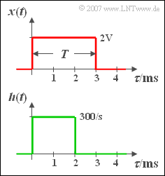
At the input of a causal LTI system (i.e. linear and time-invariant)
- with a rectangular impulse response ${h(t)}$ of duration $2 \,\text{ms}$ ,
- a rectangular pulse ${x(t)}$ of duration $T = 3 \,\text{ms}$ and amplitude $A = 2\,\text{ V}$ is applied.
The rectangular functions each start at the time $t = 0$.
In this task you are to calculate the output signal ${y(t)}$ with the help of the "Graphical Convolution".
As you can easily check, the output signal ${y(t)}$
- differs from zero only in the range between $0$ and $5 \, \text{ms}$, and
- is symmetrical at the time $t = 2.5 \, \text{ms}$.
Hints:
- This exercise belongs to the chapter "The Convolution Theorem and Operation".
- It mainly refers to the page "Graphical convolution".
- The topic of this section is also illustrated in the interactive applet "Graphical Convolution".
Questions
Solution
(1) In general, the following applies to the convolution integral:
- $$y(t) = \int_{ - \infty }^{ + \infty } {x( \tau ) \cdot h( {t - \tau } )}\hspace{0.1cm} {\rm d}\tau.$$
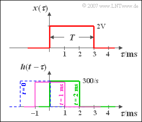
The signal value at time $t = 1 \,\text{ms}$ can be calculated as follows:
- Mirroring of the impulse response ${h(\tau)}$,
- shifting by $t = 1 \text{ ms}$ to the right (violet curve in the sketch),
- multiplication of the two functions and integration.
The product is also rectangular with the height $2 \text{ V} \cdot 300 \; \text{1/s}$ and width $1 \,\text{ms}$. This results for the area:
- $$y( {t = 1\;{\rm{ms}}} ) \hspace{0.15 cm}\underline{= 0.6\;{\rm{V}}}{\rm{.}}$$
The green rectangle illustrates the calculation of the second signal value. Now the resulting rectangle is twice as wide after the multiplication and we get:
- $$y( {t = 2\;{\rm{ms}}} ) = 2\;{\rm{V}} \cdot {\rm{300}}\;{1}/{{\rm{s}}} \cdot 2\;{\rm{ms}}\hspace{0.15 cm}\underline{={\rm{1.2}}\;{\rm{V}}}{\rm{.}}$$
(2) Because of the symmetry of ${y(t)}$ with respect to the time $t = 2.5\, \text {ms}$ holds:
- $$y( {t = 3\;{\rm{ms}}} ) = y( {t = 2\;{\rm{ms}}} ) \hspace{0.15 cm}\underline{= {\rm{1}}{\rm{.2}}\;{\rm{V}}}{\rm{,}}$$
- $$y( {t = 4\;{\rm{ms}}} ) = y( {t = 1\;{\rm{ms}}} )\hspace{0.15 cm}\underline{ = 0.6\;{\rm{V}}}{\rm{.}}$$
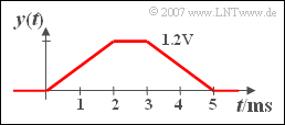
(3) Proposed solutions 1 and 3 are correct:
- In subtasks (1) and (2) the signal values were calculated at discrete time points.
- All points are to be connected by straight line segments, since the integration over rectangular functions of increasing width results in a linear course.
- This means: The output signal ${y(t)}$ is trapezoidal.
- The associated spectrum is complex and reads:
- $$Y(f) = 6 \cdot 10^{ - 3} \;{{\rm{V}}}/{{{\rm{Hz}}}} \cdot {\mathop{\rm si}\nolimits} ( {2\;{\rm{ms}}\cdot{\rm{\pi }}f} ) \cdot {\mathop{\rm si}\nolimits} ( {3\;{\rm{ms}}\cdot{\rm{\pi }}f}) \cdot {\rm{e}}^{ - {\rm{j \hspace{0.05cm}\cdot \hspace{0.05cm} 2 \hspace{0.05cm}\cdot \hspace{0.05cm}2.5\;{\rm{ms}}\hspace{0.05cm}\cdot \hspace{0.05cm} \pi }}f} .$$
- If the input pulse ${x(t)}$ would have the duration $T = 2\, \text {ms}$, the duration ${y(t)}$ would show a triangular waveform between ${t = 0}$ and $t = 4 \text { ms}$. The maximum $1.2 \, \text {V}$ would then only result at the time $t = 2 \, \text {ms}$.


