Difference between revisions of "Linear and Time Invariant Systems/Classification of the Distortions"
m (Text replacement - "”" to """) |
|||
| Line 41: | Line 41: | ||
| − | For the whole main chapter | + | For the whole main chapter "Signal Distortions and Equalisation" the following shall apply: |
*The system be '''time-invariant'''. If the input signal $x(t)$ results in the output signal $y(t)$, then a later input signal of the same form – in particular $x(t - t_0)$ – will result in the signal $y(t - t_0)$ . | *The system be '''time-invariant'''. If the input signal $x(t)$ results in the output signal $y(t)$, then a later input signal of the same form – in particular $x(t - t_0)$ – will result in the signal $y(t - t_0)$ . | ||
* '''No noise''' is considered, which is always present in real systems. For the description of these phenomena we refer to the $\rm LNTwww$–book [[Stochastische Signaltheorie]]. | * '''No noise''' is considered, which is always present in real systems. For the description of these phenomena we refer to the $\rm LNTwww$–book [[Stochastische Signaltheorie]]. | ||
| Line 127: | Line 127: | ||
*The energy of the damped and delayed signal $α · x(t - τ)$ is equal to $α^2 · E_x$ independent of the transit time $τ$ . Thus for the signal-to-distortion (power) ratio the following is applicable: | *The energy of the damped and delayed signal $α · x(t - τ)$ is equal to $α^2 · E_x$ independent of the transit time $τ$ . Thus for the signal-to-distortion (power) ratio the following is applicable: | ||
:$$\rho_{\rm D} = \frac{ \alpha^2 \cdot E_{x}}{E_{\rm D}}\hspace{0.3cm}{\rm or}\hspace{0.3cm}\rho_{\rm D}= \frac{ \alpha^2 \cdot P_{x}}{P_{\rm D}} .$$ | :$$\rho_{\rm D} = \frac{ \alpha^2 \cdot E_{x}}{E_{\rm D}}\hspace{0.3cm}{\rm or}\hspace{0.3cm}\rho_{\rm D}= \frac{ \alpha^2 \cdot P_{x}}{P_{\rm D}} .$$ | ||
| − | *The first of these two equations applies to time-limited and thus energy-limited signals, the second one to time-unlimited and thus power-limited signals according to the page [[Signal_Representation/Signal_classification#Energiebegrenzte_und_leistungsbegrenzte_Signale|Energiebegrenzte und leistungsbegrenzte Signale]] in the book | + | *The first of these two equations applies to time-limited and thus energy-limited signals, the second one to time-unlimited and thus power-limited signals according to the page [[Signal_Representation/Signal_classification#Energiebegrenzte_und_leistungsbegrenzte_Signale|Energiebegrenzte und leistungsbegrenzte Signale]] in the book "Signal Representation". |
==Linear and Nonlinear Distortions== | ==Linear and Nonlinear Distortions== | ||
Revision as of 16:22, 28 May 2021
Contents
# OVERVIEW OF THE SECOND MAIN CHAPTER #
$\text{Definition:}$ Generally, undesirable deterministic changes of a message signal by a transmission system are considered as distortions .
In addition to stochastic interferences (noise, crosstalk, etc.), such deterministic distortions are a critical limitation on transmission quality and rate for many messaging systems.
This chapter presents these distortions in a summarising way, in particular:
- the quantitative detection of such signal falsifications via the distortion power,
- the distinguishing features between nonlinear and linear distortions,
- the meaning and computation of the distortion factor in nonlinear systems and
- the effects of linear distortions of damping and phase distortions.
Further information on the topic of "distortions" as well as tasks, simulations and programming exercises can be found in
- Chapter 6: Linear Time-Invariant Systems (Programme lzi)
of the practical course "Simulation Methods in Communications Engineering". This (former) LNT course at TU Munich is based on
- the educational software package LNTsim ⇒ Link refers to the ZIP-version of the programme, and
- this practical course guide Praktikumsanleitung ⇒ Link refers to the PDF-version; Chapter 6: pages 99-118.
Prerequisites for the Entire Second Main Chapter
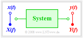
In the following, we consider a system whose input is the signal $x(t)$ with the corresponding spectrum $X(f)$ . The output signal is denoted by $y(t)$ and its spectrum by $Y(f).$
The block labelled "system" can be a part of an electrical circuit or a complete transmission system consisting of transmitter, channel and receiver.
For the whole main chapter "Signal Distortions and Equalisation" the following shall apply:
- The system be time-invariant. If the input signal $x(t)$ results in the output signal $y(t)$, then a later input signal of the same form – in particular $x(t - t_0)$ – will result in the signal $y(t - t_0)$ .
- No noise is considered, which is always present in real systems. For the description of these phenomena we refer to the $\rm LNTwww$–book Stochastische Signaltheorie.
- No detailed knowledge about the system is assumed. In the following, all system properties are derived from the signals $x(t)$ and $y(t)$ or their spectra alone.
- In particular, no specifications are given with regards to linearity for the time being. The "system" can be linear (prerequisite for the application of the superposition principle) or non-linear.
- Not all system properties are discernible from a single test signal $x(t)$ and its response $y(t)$ . Therefore, sufficiently many test signals must be used for evaluation.
In the following, we will classify transmission systems in more detail in this respect.
Ideal and Distortion-free System
$\text{Definition:}$ One deals with an ideal system if the output signal $y(t)$ is exactly equal to the input signal $x(t)$ :
- $$y(t) \equiv x(t).$$
It should be noted that such an ideal system does not exist in reality even if statistical disturbances and noise processes, that always exist but are not considered in this book, are disregarded. Every transmission medium exhibits losses (damping) and transit times. Even if these physical phenomena are very small, they are never zero. It is therefore necessary to introduce a somewhat less strict quality characteristic.
$\text{Definition:}$ A distortion-free system exists if the following condition is fulfilled:
- $$y(t) = \alpha \cdot x(t - \tau).$$
Here, $α$ describes the damping factor and $τ$ the transit time.
If this condition is not met, the system is said to be distortive.
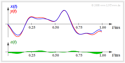
$\text{Example 1:}$ The following diagram shows the input signal $x(t)$ and the output signal $y(t)$ of a nonideal but distortion-free system. The system parameters are $α = 0.8$ and $τ = 0.25 \ \rm ms$.
Note:
- The damping factor $α$ can be completely reversed by a receiver-side gain of $1/α = 1.25$, but it must be taken into account that this also increases any noise.
- However, the transit time $τ$ cannot be compensated due to Kausalitätsgründen . It now depends on the application whether such a transit time is subjectively perceived as disturbing or not.
For example, even with a transit time of one second the (unidirectional) TV broadcast of an event is still described as "live". In contrast to this, transit times of $\text{300 ms}$ are already perceived as very disturbing in bidirectional communication – for example, a telephone call. You either wait for the other person to react or both participants interrupt each other.
Quantitative Measure of Signal Distortion
We now consider a distortive system on the basis of the input and output signal. In doing so, we assume that apart from the signal distortions there is no additional damping factor $α$ which is constant for all frequencies and no additional transit time $τ$ that is constant for all frequencies. These conditions are fulfilled for the signal sections sketched below.
In addition to the signals $x(t)$ and $y(t)$ , the difference signal is also shown in the diagram:
- $$\varepsilon(t) = y(t) - x(t).$$
As a quantitative measure of the strength of distortions, for example, the squared mean of this difference signal is applicable:
- $$\overline{\varepsilon^2(t)} = \frac{1}{T_{\rm M}} \cdot \int_{ 0 }^{ T_{\rm M}} {\varepsilon^2(t) }\hspace{0.1cm}{\rm d}t\hspace{0.4cm} \left( = P_{\rm V} \right).$$
The following should be noted about this equation:
- The measurement time $T_{\rm M}$ must be chosen sufficiently large. Actually, this equation should be formulated as a limit process.
- The squared mean mentioned above is often also called mean squared error $\rm (MSE)$ or distortion power $P_{\rm D}$ .
- If $x(t)$ and $y(t)$ are voltage signals, then $P_{\rm D}$ has the unit of ${\rm V}^2$, meaning the power is related to the resistance $R = 1 \ Ω$ according to the above definition.
$\text{Definition:}$ Making use of the power (based on $R = 1 \ Ω$ ) $P_x$ of the input signal $x(t)$ the signal–to–distortion (power) ratio can be given as:
- $$\rho_{\rm D} = \frac{ P_{x} }{P_{\rm D} } \hspace{0.3cm} \Rightarrow \hspace{0.3cm} 10 \cdot \lg \hspace{0.1cm}\rho_{\rm D} = 10 \cdot \lg \hspace{0.1cm}\frac{ P_{x} }{P_{\rm D} }\hspace{0.3cm} \left( {\rm in \hspace{0.15cm} dB} \right).$$
For the signals shown in the diagram above $P_x = 4 \ {\rm V}^2$, $P_{\rm D} = 0.04 \ {\rm V}^2$ and thus $10 \cdot {\rm lg} \ ρ_{\rm D} = 20 \ \rm dB$ hold.
We reference the interactive applet Lineare Verzerrungen periodischer Signale.
Significance of Damping and Transit Time
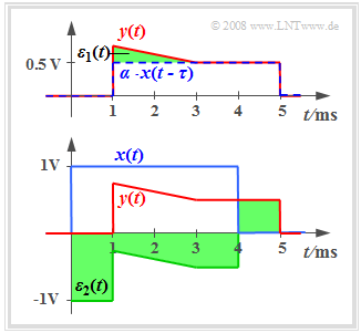
The equations given on the last page do not result in applicable statements if the system is additionanlly affected by an attenuation $α$ and/or transit time $τ$ . The diagram shows the attenuated, delayed and distorted signal
- $$y(t) = \alpha \cdot x(t - \tau) + \varepsilon_1(t).$$
The term $ε_1(t)$ summarises all distortions. It can be seen from the green area that the error signal $ε_1(t)$ is relatively small.
In contrast to this, if the attenuation $α$ and transit time $τ$ are unknwon, the following should be noted:
- The error signal $ε_2(t) = y(t) - x(t)$ determined in this way is relatively large despite small distortions $ε_1(t)$ .
- Here, instead of the distortion power the distortion energy must be considered because $x(t)$ and $y(t)$ are energy-limited signals.
- The distortion energy is obtained by varying the unknown quantities $α$ and $τ$ and thus finding the minimum of the mean squared error:
- $$E_{\rm D} = \min_{\alpha, \ \tau} \int_{ - \infty }^{ + \infty} {\big[y(t) - \left(\alpha \cdot x(t - \tau) \right) \big]^2}\hspace{0.1cm}{\rm d}t.$$
- The energy of the damped and delayed signal $α · x(t - τ)$ is equal to $α^2 · E_x$ independent of the transit time $τ$ . Thus for the signal-to-distortion (power) ratio the following is applicable:
- $$\rho_{\rm D} = \frac{ \alpha^2 \cdot E_{x}}{E_{\rm D}}\hspace{0.3cm}{\rm or}\hspace{0.3cm}\rho_{\rm D}= \frac{ \alpha^2 \cdot P_{x}}{P_{\rm D}} .$$
- The first of these two equations applies to time-limited and thus energy-limited signals, the second one to time-unlimited and thus power-limited signals according to the page Energiebegrenzte und leistungsbegrenzte Signale in the book "Signal Representation".
Linear and Nonlinear Distortions
A distinction is made between linear and nonlinear distortions:
If the system is linear and time-invariant $(\rm LTI)$, then it is fully characterised by its Frequenzgang $H(f)$ and the following can be stated:
- According to the $H(f)$–definition the following holds for the output spectrum: $Y(f)=X(f) · H(f)$. As a consequence according to the calculation rules of multiplication, $Y(f)$ cannot contain any frequency components that are not already contained in $X(f)$ .
- The inverse implies: The output signal $y(t)$ can include any frequency $f_0$ already contained in the input signal $x(t)$ . The prerequisite is therefore that $X(f_0) ≠ 0$ holds.
- For an LTI-system the absolute bandwidth $(B_y)$ of the output signal is never greater than the bandwidth $(B_x)$ of the input signal: $B_y \le B_x .$
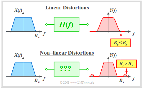
$\text{Conclusion:}$ The differences between linear and non-linear distortions are illustrated by the following diagram:
- In the above diagram $B_y = B_x$ holds. There are linear distortions because in this frequency band $X(f)$ and $Y(f)$ differ.
- A band limitation $(B_y < B_x)$ is a special form of linear distortion, which will be discussed in the chapter after next .
- The below diagram shows an example of nonlinear distortions $(B_y > B_x)$. For such a system no frequency response $H(f)$ can be given.
- Descriptive quantities applicable for nonlinear systems will be explained in the next chapter nonlinear distortions .
In most real transmission channels both linear and nonlinear distortions occur. However, for a whole range of problems the precise separation of the two types of distortions is essential. In [Kam04][1] a corresponding substitute model is shown.
We refer here to the learning video Lineare und nichtlineare Verzerrungen .
Exercises for the Chapter
Aufgabe 2.1: Linear? - Nichtlinear?
Aufgabe 2.1Z: Verzerrung und Entzerrung
Aufgabe 2.2: Verzerrungsleistung
Aufgabe 2.2Z: Nochmals Verzerrungsleistung
Bibliography
- ↑ Kammeyer, K.D.: Nachrichtenübertragung. Stuttgart: B.G. Teubner, 4. Auflage, 2004.


