Difference between revisions of "Aufgaben:Exercise 2.5: Residual Redundancy with LZW Coding"
| Line 20: | Line 20: | ||
whereby we have restricted ourselves to sequence lengths $N ≤ 50000$ in the simulation. | whereby we have restricted ourselves to sequence lengths $N ≤ 50000$ in the simulation. | ||
| − | The "relative redundancy of the output sequence" – simplified called | + | The "relative redundancy of the output sequence" – simplified called "residual redundancy" – can be calculated from |
* the length $N$ of the input sequence, | * the length $N$ of the input sequence, | ||
* the length $L(N)$ of the output sequence and | * the length $L(N)$ of the output sequence and | ||
| Line 38: | Line 38: | ||
:$$K(N) = {L(N) }/{N} \hspace{0.05cm},$$ | :$$K(N) = {L(N) }/{N} \hspace{0.05cm},$$ | ||
| − | In the [[Information_Theory/Komprimierung_nach_Lempel,_Ziv_und_Welch#Quantitative_statements_on_asymptotic_optimality|theory section]] it was shown that the residual redundancy $r(n)$ is | + | In the [[Information_Theory/Komprimierung_nach_Lempel,_Ziv_und_Welch#Quantitative_statements_on_asymptotic_optimality|theory section]] it was shown that the residual redundancy $r(n)$ is well approximated by the function |
:$$r\hspace{0.05cm}'(N) =\frac {A}{{\rm lg}\hspace{0.1cm}(N)} | :$$r\hspace{0.05cm}'(N) =\frac {A}{{\rm lg}\hspace{0.1cm}(N)} | ||
\hspace{0.5cm}{\rm mit}\hspace{0.5cm} A = 4 \cdot {r(N = 10000)} | \hspace{0.5cm}{\rm mit}\hspace{0.5cm} A = 4 \cdot {r(N = 10000)} | ||
\hspace{0.05cm}.$$ | \hspace{0.05cm}.$$ | ||
| − | + | ||
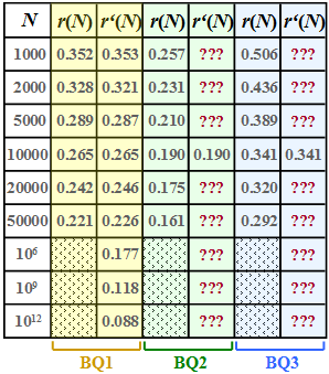
*This approximation $r\hspace{0.05cm}'(N)$ is given for $\rm BQ1$ in the second column of the table above. | *This approximation $r\hspace{0.05cm}'(N)$ is given for $\rm BQ1$ in the second column of the table above. | ||
| Line 96: | Line 96: | ||
| − | {According to this result, what source entropy $H$ could $\rm BQ3$ ? < | + | {According to this result, what source entropy $H$ could $\rm BQ3$ ? <u>Hint:</u> Exactly one answer is correct. |
|type="()"} | |type="()"} | ||
- $H = 1.00 \ \rm bit/source symbol$, | - $H = 1.00 \ \rm bit/source symbol$, | ||
Revision as of 11:52, 10 August 2021
We assume here a binary input sequence of length $N$ and consider three different binary sources:
- $\rm BQ1$: Symbol probabilities $p_{\rm A} = 0.89$ and $p_{\rm B} = 0.11$, i.e. different
⇒ entropy $H = 0.5\text{ bit/source symbol}$ ⇒ the source is redundant. - $\rm BQ2$: $p_{\rm A} = p_{\rm B} = 0.5$ (equally probable)
⇒ entropy $H = 1\text{ bit/source symbol}$ ⇒ the source is redundancy-free. - $\rm BQ3$: There is no concrete information on the statistics here.
In subtask (6) you are to estimate the entropy $H$ of this source.
For these three sources, the respective "residual redundancy" $r(N)$ was determined by simulation, which remains in the binary sequence after Lempel–Ziv–Welch coding.
The results are shown in the first column of the above table for the sources
- $\rm BQ1$ (yellow background),
- $\rm BQ2$ (green background) and
- $\rm BQ3$ (blue background)
whereby we have restricted ourselves to sequence lengths $N ≤ 50000$ in the simulation.
The "relative redundancy of the output sequence" – simplified called "residual redundancy" – can be calculated from
- the length $N$ of the input sequence,
- the length $L(N)$ of the output sequence and
- the entropy $H$
in the following way:
- $$r(N) = \frac{L(N) - N \cdot H}{L(N)}= 1 - \frac{ N \cdot H}{L(N)}\hspace{0.05cm}.$$
This takes into account that with perfect source coding the length of the output sequence could be lowered to the value $L_{\rm min} = N · H$ .
- With non-perfect source coding, $L(n) - N · H$ gives the remaining redundancy (with the pseudo–unit "bit").
- After dividing by $L(n)$, one obtains the relative redundancy $r(n)$ with the value range between zero and one; $r(n)$ should be as small as possible.
A second parameter for measuring the efficiency of LZW coding is the "compression factor" $K(N)$ as the quotient of the lengths of the output and input sequences, which should also be very small:
- $$K(N) = {L(N) }/{N} \hspace{0.05cm},$$
In the theory section it was shown that the residual redundancy $r(n)$ is well approximated by the function
- $$r\hspace{0.05cm}'(N) =\frac {A}{{\rm lg}\hspace{0.1cm}(N)} \hspace{0.5cm}{\rm mit}\hspace{0.5cm} A = 4 \cdot {r(N = 10000)} \hspace{0.05cm}.$$
- This approximation $r\hspace{0.05cm}'(N)$ is given for $\rm BQ1$ in the second column of the table above.
- In subtasks (4) and (5) you are to make the approximation for sources $\rm BQ2$ and $\rm BQ3$ .
Hints:
- The task belongs to the chapter Compression according to Lempel, Ziv and Welch.
- In particular, reference is made to the pages
- The descriptive variables $K(N)$ and $r(N)$ are deterministically related.
Questions
Solution
- Thus
- $$A = 4 \cdot r(N = 10000) =4 \cdot {0.265} \hspace{0.15cm}\underline{= 1.06} \hspace{0.05cm}. $$
(2) From the relationship ${A}/{\rm lg}\hspace{0.1cm}(N) ≤ 0.05$ ⇒ ${A}/{\rm lg}\hspace{0.1cm}(N) = 0.05$ it follows:
- $${{\rm lg}\hspace{0.1cm}N_{\rm 2}} = \frac{A}{0.05} = 21.2 \hspace{0.3cm}\Rightarrow\hspace{0.3cm} N_{\rm 2} = 10^{21.2} \hspace{0.15cm}\underline{= 1.58 \cdot 10^{21}} \hspace{0.05cm}.$$
(3) In general, $r(N) = 1 - {H}/{K(N)} \hspace{0.05cm}.$
- $\rm BQ1$ has entropy $H = 0.5$ bit/symbol.
- It follows that because $r(N) ≈ r\hspace{0.05cm}'(N)$ für $K(N_3) = 0.6$:
- $$r(N_{\rm c}) = 1 - \frac{0.5}{0.6} = 0.167 \hspace{0.1cm}\Rightarrow\hspace{0.1cm} {\rm lg}\hspace{0.1cm}N_{\rm 3} = \frac{A}{0.167} = 6.36 \hspace{0.1cm}\Rightarrow\hspace{0.1cm} N_{\rm 3} = 10^{6.36} \hspace{0.15cm}\underline{= 2.29 \cdot 10^{6}} \hspace{0.05cm}.$$
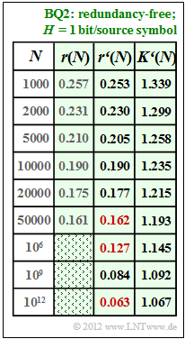
(4) For $N = 10000$ gilt $r(N) ≈ r\hspace{0.05cm}'(N) = 0.19$:
- $$\frac{A}{{\rm lg}\hspace{0.1cm}10000} = 0.19 \hspace{0.3cm}\Rightarrow\hspace{0.3cm} A = 0.19 \cdot 4 = 0.76 \hspace{0.05cm}. $$
- The results are summarised in the table opposite.
- One can see the very good agreement between $r(N)$ and $r\hspace{0.05cm}'(N)$.
- The numerical values sought are marked in red in the table:
$$r'(N = 50000)\hspace{0.15cm}\underline{ = 0.162},\hspace{0.3cm}r'(N = 10^{6})\hspace{0.15cm}\underline{ = 0.127},\hspace{0.3cm} r'(N = 10^{12})\hspace{0.15cm}\underline{ = 0.063}.$$
- For the compression factor, (the apostrophe indicates that the approximation $r\hspace{0.05cm}'(N)$ was assumed):
- $$K\hspace{0.05cm}'(N) = \frac{1}{1 - r\hspace{0.05cm}'(N)}\hspace{0.05cm}.$$
- Thus, for the length of the LZW output string:
- $$L\hspace{0.05cm}'(N) = K\hspace{0.05cm}'(N) \cdot N = \frac{N}{1 - r\hspace{0.05cm}'(N)}\hspace{0.05cm}.$$
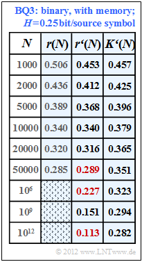
(5) Following a similar procedure as in subtask (4) we obtain the fitting parameter $\rm BQ3$ for the binary source $A = 1.36$ and from this the results according to the table with a blue background.
Hint: The last column of this table is only understandable with knowledge of subtask (6) . There it is shown that the source $\rm BQ3$ has the entropy $H = 0.25$ bit/source symbol.
- In this case, the following applies to the compression factor:
- $$K\hspace{0.05cm}'(N) = \frac{H}{1 - r\hspace{0.05cm}'(N)} = \frac{0.25}{1 - r'(N)} \hspace{0.05cm}.$$
- Thus, for the values of residual redundancy we are looking for, we obtain:
- $$r\hspace{0.05cm}'(N = 50000)\hspace{0.15cm}\underline{ = 0.289},\hspace{0.3cm}r\hspace{0.05cm}'(N = 10^{6})\hspace{0.15cm}\underline{ = 0.227},\hspace{0.3cm} r\hspace{0.05cm}'(N = 10^{12})\hspace{0.15cm}\underline{ = 0.113}.$$
- Thus, for $N = 10^{12}$ , the compression factor $(0.282)$ still deviates significantly from the entropy $(0.25)$ which can only be achieved for $N \to \infty$ (source coding theorem).
(6) The individual approximations $r\hspace{0.05cm}'(N)$ differ only by the parameter $A$. Here we found:
- Source $\rm BQ1$ with $H = 0.50$ ⇒ $A = 1.06$ ⇒ according to the specification sheet,
- Source $\rm BQ2$ with $H = 1.00$ ⇒ $A = 0.76$ ⇒ see subtask (4),
- Source $\rm BQ3$ $(H$ unknown$)$: $A = 4 · 0.34 =1.36$ ⇒ corresponding to the last column in the table.
- Obviously, the smaller the entropy $H$ the larger the adjustment factor $A$ (and vice versa).
- Since exactly one solution is possible, $H = 0.25$ bit/source symbol must be correct ⇒ answer 4.
- In fact, the probabilities $p_{\rm A} = 0.96$ and $p_{\rm B} = 0.04$ ⇒ $H ≈ 0.25$ were used in the simulation for source $\rm BQ3$ .


