Difference between revisions of "Aufgaben:Exercise 1.4Z: Everything Rectangular"
From LNTwww
| (27 intermediate revisions by 4 users not shown) | |||
| Line 1: | Line 1: | ||
| − | {{quiz-Header|Buchseite= | + | {{quiz-Header|Buchseite=Linear_and_Time_Invariant_Systems/System_Description_in_Time_Domain}} |
| − | [[File:P_ID834__LZI_Z_1_4.png |right|frame| | + | [[File:P_ID834__LZI_Z_1_4.png |right|frame|Periodic rectangular signal and <br>filter with rectangular impulse response]] |
| − | + | We consider the periodic rectangular signal $x(t)$ , whose periodic duration is $T_0 = 2T$ , according to the sketch above. | |
| − | * | + | *This signal has spectral components at the fundamental frequency $f_0 = 1/T_0 = 1/(2T)$ and at all odd multiples thereof, that is, at $3f_0$, $5f_0,$ and so on. In addition, there is a direct component. |
| − | |||
| + | *For this purpose, we consider two filters $\rm A$ and $\rm B$ each with rectangular impulse response $h_{\rm A}(t)$ with duration $6T$ and $h_{\rm B}(t)$ with duration $5T$, respectively. | ||
| + | *The heights of the two impulse responses are such that the areas of the rectangles each add up to $1$ . | ||
| Line 13: | Line 14: | ||
| − | '' | + | |
| − | * | + | |
| − | * | + | ''Please note:'' |
| − | * | + | *The exercise belongs to the chapter [[Linear_and_Time_Invariant_Systems/System_Description_in_Time_Domain|System Description in Time Domain]]. |
| − | + | *For information on convolution, see the chapter [[Signal_Representation/The_Convolution_Theorem_and_Operation|convolution theorem and operation]] in the book "Signal Representation”. | |
| + | *We also refer you to the interactive applet [[Applets:Zur_Verdeutlichung_der_grafischen_Faltung|Zur Verdeutlichung der graphischen Faltung]]. | ||
| + | |||
| − | === | + | ===Questions=== |
<quiz display=simple> | <quiz display=simple> | ||
| − | { | + | {Compute the output signal $y_{\rm A}(t)$ of the filter $\rm A$, in particular the values at $t = 0$ and $t = T$. |
|type="{}"} | |type="{}"} | ||
$y_{\rm A}(t = 0) \ =\ $ { 1 3% } $\rm V$ | $y_{\rm A}(t = 0) \ =\ $ { 1 3% } $\rm V$ | ||
| Line 30: | Line 33: | ||
| − | { | + | {Give the absolute value function $|H_{\rm A}(f)|$ . What value is obtained at frequency $f = f_0$? <br>Interpret the result of the subtask '''(1)'''. |
|type="{}"} | |type="{}"} | ||
$|H_{\rm A}(f = f_0)| \ =\ $ { 0. } | $|H_{\rm A}(f = f_0)| \ =\ $ { 0. } | ||
| − | { | + | {Compute the output signal $y_{\rm B}(t)$ of the filter $\rm B$, in particular the values at $t = 0$ and $t = T$. |
|type="{}"} | |type="{}"} | ||
$y_{\rm B}(t = 0) \ =\ $ { 0.8 3% } $\rm V$ | $y_{\rm B}(t = 0) \ =\ $ { 0.8 3% } $\rm V$ | ||
| Line 41: | Line 44: | ||
| − | { | + | {What is the absolute value function $|H_{\rm B}(f)|$, especially at frequencies $f = f_0$ and $f = 3 · f_0$? <br>Use this to interpret the result of the subtask '''(3)'''. |
|type="{}"} | |type="{}"} | ||
$|H_{\rm B}(f = f_0)| \ =\ $ { 0.127 5% } | $|H_{\rm B}(f = f_0)| \ =\ $ { 0.127 5% } | ||
| Line 48: | Line 51: | ||
</quiz> | </quiz> | ||
| − | === | + | ===Solution=== |
{{ML-Kopf}} | {{ML-Kopf}} | ||
| − | '''1 | + | '''(1)''' The output signal is the result of the convolution operation between $x(t)$ and $h_{\rm A}(t)$: |
| − | $$y_{\rm A}(t) = x (t) * h_{\rm A} (t) = \int_{ - \infty }^{ + \infty } {x ( \tau )} \cdot h_{\rm A} ( {t - \tau } ) \hspace{0.1cm}{\rm d}\tau.$$ | + | :$$y_{\rm A}(t) = x (t) * h_{\rm A} (t) = \int_{ - \infty }^{ + \infty } {x ( \tau )} \cdot h_{\rm A} ( {t - \tau } ) \hspace{0.1cm}{\rm d}\tau.$$ |
| − | + | *Because of the rectangular function and the duration $6T$ this can also be written as follows: | |
| − | $$y_{\rm A}(t) = \frac{1}{6T}\cdot \int_{t-6T}^{t}x(\tau)\hspace{0.15cm} {\rm d}\tau.$$ | + | :$$y_{\rm A}(t) = \frac{1}{6T}\cdot \int_{t-6T}^{t}x(\tau)\hspace{0.15cm} {\rm d}\tau.$$ |
| − | + | *It can be seen that this equation gives the same result $y_{\rm A}(t) \rm \underline{\: = 1V}$ for all $t$ . | |
| + | |||
| − | '''2 | + | '''(2)''' The magnitude of the frequency response is $|H_{\rm A}(f)| = |{\rm si}(\pi \cdot f \cdot 6T)|.$ This has zeros at an interval of $1/(6T)$ . |
| − | * | + | *So, there are also zeros at $f_0$, $3f_0$, $5f_0$ etc., respectively. |
| − | * | + | *In particular, $|H_{\rm A}(f = f_0)| \underline{\: = 0}$ holds, too. |
| − | * | + | *From the spectrum $X(f)$ only the direct component $1 \hspace{0.05cm} \rm V$ remains unchanged. |
| + | *In contrast to this, all other spectral lines in $Y_{\rm A}(f)$ are no longer included. | ||
| − | + | [[File:P_ID836__LZI_Z_1_4_c.png | Graphical illustration of the convolution operation| rechts|frame]] | |
| − | + | '''(3)''' Analogous to the subtask '''(1)''' for the output signal the following can be recorded: | |
| − | $$y_{\rm B}(t) = \frac{1}{5T}\cdot \int_{t-5T}^{t}x(\tau)\hspace{0.15cm} {\rm d}\tau.$$ | + | :$$y_{\rm B}(t) = \frac{1}{5T}\cdot \int_{t-5T}^{t}x(\tau)\hspace{0.15cm} {\rm d}\tau.$$ |
| − | + | *This results in a triangular shape fluctuating around the mean $1 \ \rm V$ ⇒ see bottom graph. | |
| − | * | + | *Since two rectangles and three gaps each are covered by the integration interval, the following holds for $t = 0, t = 2T,$ etc.: |
| − | + | :$$y_{\rm B}(t) = \frac{2\,{\rm V} \cdot 2T }{5T} \hspace{0.15cm}\underline{= 0.8\,{\rm V} =y_{\rm B}(t=0) }.$$ | |
| − | * | + | *For $t = T,\ 3T, \ 5T, $ etc., there are three rectangles and two gaps each to be considered: One obtains: |
| + | :$$y_{\rm B}(t) \underline{\: = 1.2 \: {\rm V}=y_{\rm B}(t=T)}.$$ | ||
| − | |||
| − | |||
| − | + | '''(4)''' The magnitude function is generally or at frequencies $f = f_0 = 1/(2T)$ and $f = 3f_0$: | |
| + | :$$\begin{align*} |H_{\rm B}(f)| & = |{\rm si}(\pi \cdot f \cdot 5T)|, \\ |H_{\rm B}(f = f_0)| & = |{\rm si}(\pi \frac{5T}{2T})| = |{\rm si}(2.5\pi )| = \frac{1}{2.5 \pi} \hspace{0.15cm}\underline{= 0.127}, \\ |H_{\rm B}(f = 3f_0)| & = |{\rm si}(7.5\pi )| = \frac{1}{7.5 \pi} \hspace{0.15cm}\underline{=0.042}.\end{align*}$$ | ||
| − | + | Interpretation: | |
| + | *The spectral components of the rectangular signal at $f_0, 3f_0,$ etc., although now no longer suppressed, are increasingly attenuated as the frequency increases, in such a way that the rectangular curve is converted into a periodic triangular signal. The direct component $(1 \hspace{0.05cm} \rm V)$ remains unchanged here, too. | ||
| + | *Thus, both filters provide the average value of the input signal. For the signal $x(t)$ at hand the filter $\rm A$ is more suitable than the filter $\rm B$ for the determination of the mean value, because for the former the length of the impulse response is a multiple of the period $T_0 = 2T$ . | ||
| + | *If this condition – as with the filter $\rm B$ – is not fulfilled, an error signal (triangular in this example) is still superimposed on the mean value. | ||
{{ML-Fuß}} | {{ML-Fuß}} | ||
| Line 83: | Line 91: | ||
| − | [[Category: | + | [[Category:Linear and Time-Invariant Systems: Exercises|^1.2 System Description in Time Domain^]] |
Latest revision as of 19:49, 5 September 2021
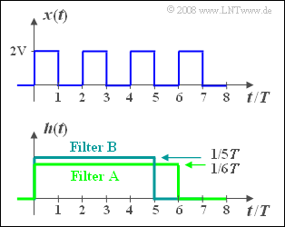
We consider the periodic rectangular signal $x(t)$ , whose periodic duration is $T_0 = 2T$ , according to the sketch above.
- This signal has spectral components at the fundamental frequency $f_0 = 1/T_0 = 1/(2T)$ and at all odd multiples thereof, that is, at $3f_0$, $5f_0,$ and so on. In addition, there is a direct component.
- For this purpose, we consider two filters $\rm A$ and $\rm B$ each with rectangular impulse response $h_{\rm A}(t)$ with duration $6T$ and $h_{\rm B}(t)$ with duration $5T$, respectively.
- The heights of the two impulse responses are such that the areas of the rectangles each add up to $1$ .
Please note:
- The exercise belongs to the chapter System Description in Time Domain.
- For information on convolution, see the chapter convolution theorem and operation in the book "Signal Representation”.
- We also refer you to the interactive applet Zur Verdeutlichung der graphischen Faltung.
Questions
Solution
(1) The output signal is the result of the convolution operation between $x(t)$ and $h_{\rm A}(t)$:
- $$y_{\rm A}(t) = x (t) * h_{\rm A} (t) = \int_{ - \infty }^{ + \infty } {x ( \tau )} \cdot h_{\rm A} ( {t - \tau } ) \hspace{0.1cm}{\rm d}\tau.$$
- Because of the rectangular function and the duration $6T$ this can also be written as follows:
- $$y_{\rm A}(t) = \frac{1}{6T}\cdot \int_{t-6T}^{t}x(\tau)\hspace{0.15cm} {\rm d}\tau.$$
- It can be seen that this equation gives the same result $y_{\rm A}(t) \rm \underline{\: = 1V}$ for all $t$ .
(2) The magnitude of the frequency response is $|H_{\rm A}(f)| = |{\rm si}(\pi \cdot f \cdot 6T)|.$ This has zeros at an interval of $1/(6T)$ .
- So, there are also zeros at $f_0$, $3f_0$, $5f_0$ etc., respectively.
- In particular, $|H_{\rm A}(f = f_0)| \underline{\: = 0}$ holds, too.
- From the spectrum $X(f)$ only the direct component $1 \hspace{0.05cm} \rm V$ remains unchanged.
- In contrast to this, all other spectral lines in $Y_{\rm A}(f)$ are no longer included.
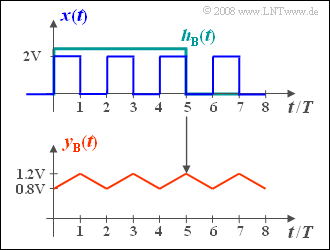
(3) Analogous to the subtask (1) for the output signal the following can be recorded:
- $$y_{\rm B}(t) = \frac{1}{5T}\cdot \int_{t-5T}^{t}x(\tau)\hspace{0.15cm} {\rm d}\tau.$$
- This results in a triangular shape fluctuating around the mean $1 \ \rm V$ ⇒ see bottom graph.
- Since two rectangles and three gaps each are covered by the integration interval, the following holds for $t = 0, t = 2T,$ etc.:
- $$y_{\rm B}(t) = \frac{2\,{\rm V} \cdot 2T }{5T} \hspace{0.15cm}\underline{= 0.8\,{\rm V} =y_{\rm B}(t=0) }.$$
- For $t = T,\ 3T, \ 5T, $ etc., there are three rectangles and two gaps each to be considered: One obtains:
- $$y_{\rm B}(t) \underline{\: = 1.2 \: {\rm V}=y_{\rm B}(t=T)}.$$
(4) The magnitude function is generally or at frequencies $f = f_0 = 1/(2T)$ and $f = 3f_0$:
- $$\begin{align*} |H_{\rm B}(f)| & = |{\rm si}(\pi \cdot f \cdot 5T)|, \\ |H_{\rm B}(f = f_0)| & = |{\rm si}(\pi \frac{5T}{2T})| = |{\rm si}(2.5\pi )| = \frac{1}{2.5 \pi} \hspace{0.15cm}\underline{= 0.127}, \\ |H_{\rm B}(f = 3f_0)| & = |{\rm si}(7.5\pi )| = \frac{1}{7.5 \pi} \hspace{0.15cm}\underline{=0.042}.\end{align*}$$
Interpretation:
- The spectral components of the rectangular signal at $f_0, 3f_0,$ etc., although now no longer suppressed, are increasingly attenuated as the frequency increases, in such a way that the rectangular curve is converted into a periodic triangular signal. The direct component $(1 \hspace{0.05cm} \rm V)$ remains unchanged here, too.
- Thus, both filters provide the average value of the input signal. For the signal $x(t)$ at hand the filter $\rm A$ is more suitable than the filter $\rm B$ for the determination of the mean value, because for the former the length of the impulse response is a multiple of the period $T_0 = 2T$ .
- If this condition – as with the filter $\rm B$ – is not fulfilled, an error signal (triangular in this example) is still superimposed on the mean value.

