Aufgaben:Exercise 4.1Z: Calculation of Moments

• Return to book

Exponential PDF (top),
Laplace PDF (bottom)

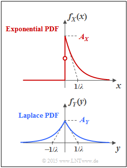
The upper graph shows the probability density function  $\rm (PDF)$  of the  exponential distribution:

$$f_X(x) = \left\{ \begin{array}{c} A_{ X} \cdot {\rm e}^{-\lambda \hspace{0.05cm} \cdot \hspace{0.05cm}x} \\ A_{ X}/2 \\ 0 \\ \end{array} \right. \begin{array}{*{20}c} {\rm{f\ddot{u}r}} \hspace{0.1cm}x>0, \\ {\rm{f\ddot{u}r}} \hspace{0.1cm}x=0, \\ {\rm{f\ddot{u}r}} \hspace{0.1cm}x<0. \\ \end{array}$$

Drawn below is the PDF of the  Laplace distribution, which can be specified for all  $y$–values as follows:

$$f_Y(y) = A_{ Y} \cdot {\rm e}^{-\lambda \hspace{0.05cm} \cdot \hspace{0.05cm} |\hspace{0.03cm}y\hspace{0.03cm}|}\hspace{0.05cm}.$$

The two value-continuous random variables  $X$  and  $Y$  are to be compared with respect to the following characteristics:

• The linear mean  $m_1$  (first order moment),
• the second order moment   ⇒   $m_2$,
• the variance  $\sigma^2 = m_2 - m_1^2$   ⇒   Steiner's theorem,
• the standard deviation  $\sigma$.

Hints:

• The task belongs to the chapter  Differential Entropy.
• Useful hints for solving this task and further information on continuous-valued random variables can be found in the third chapter "Continuous Random Variables" of the book  Theory of Stochastic Signals.

• Also given are the two indefinite integrals:

$$\int \hspace{-0.01cm} x \cdot {\rm e}^{-\lambda \hspace{0.05cm}\cdot \hspace{0.05cm}x}\hspace{0.1cm}{\rm d}x = \frac{{\rm e}^{-\lambda \hspace{0.05cm}\cdot \hspace{0.05cm}x}}{(-\lambda)^2}\cdot(-\lambda \cdot x-1)\hspace{0.05cm}, $$

$$\int \hspace{-0.01cm} x^2 \cdot {\rm e}^{-\lambda \hspace{0.05cm}\cdot \hspace{0.05cm}x}\hspace{0.1cm}{\rm d}x = {\rm e}^{-\lambda \hspace{0.05cm}\cdot \hspace{0.05cm}x}\cdot (\frac{x^2}{-\lambda} - \frac{2x}{\lambda^2} + \frac{2}{\lambda^3}) \hspace{0.05cm}. $$

Questions

1

What is the maximum value  $A_X$  of the PDF  $f_X(x)$?

	$A_X = \lambda/2$,
	$A_X = \lambda$,
	$A_X = 1/\lambda$.

2

What is the maximum value  $A_Y$  of the PDF  $f_Y(y)$?

	$A_Y = \lambda/2$,
	$A_Y = \lambda$,
	$A_Y = 1/\lambda$.

3

Is there an argument  $z$, such that  $f_X(z) = f_Y(z)$ ?

	Yes.
	No.

4

Which statements are true about the characteristics of the exponential distribution?

	The linear mean is  $m_1 = 1/\lambda$.
	The root mean square is  $m_2 = 2/\lambda^2$.
	The variance is  $\sigma^2 = 1/\lambda^2$.

5

Which statements are true about the characteristics of the Laplace distribution?

	The linear mean is  $m_1 = 1/\lambda$.
	The root mean square is  $m_2 = 2/\lambda^2$.
	The variance is  $\sigma^2 = 1/\lambda^2$.

6

With what probabilities does the random variable  $(X$  or   $Y)$  differ from the respective mean in amount by more than the dispersion  $\sigma$?

$\text{Exponential:}\; \;{\rm Pr}( |X - m_X| > \sigma_X) \ = \ $

$\text{Laplace:}\; \;{\rm Pr}( |Y - m_Y| > \sigma_Y) \ = \ $

Solution

Solution

(1)  Proposed solution 2 is correct:

• The area under the PDF must always be  $1$ .  It follows for the exponential distribution:

$$A_{X} \cdot\int_{0}^{\infty} \hspace{-0.01cm} {\rm e}^{-\lambda \hspace{0.05cm}\cdot \hspace{0.05cm}x}\hspace{0.1cm}{\rm d}x = A_{X} \cdot (-1/\lambda)\cdot\big [{\rm e}^{-\lambda \hspace{0.05cm}\cdot \hspace{0.05cm}x}\big ]_{0}^{\infty} = A_{X} \cdot (1/\lambda) \stackrel{!}{=} 1 \hspace{0.3cm} \Rightarrow\hspace{0.3cm} A_{X} = \lambda \hspace{0.05cm}. $$

(2)  Proposed solution 1 is correct:

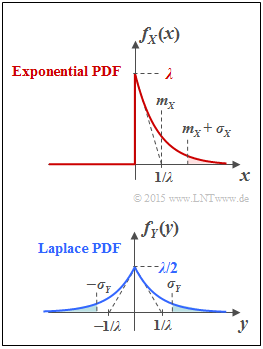
• From the graph on the information page, we can see that the height  $A_Y$  of the Laplace PDF is only half as large as the maximum of the exponential PDF:

$$A_Y = \lambda/2.$$

(3)  Correct is YES,  although for  $z \ne 0$  always  $f_X(z) = f_Y(z)$.   Let us now consider the special case  $z= 0$:

• For the Laplace PDF:  $f_Y(y = 0) = \lambda/2$.
• For the exponential PDF,  the left-hand and right-hand limits differ for  $x \to 0$.
• The PDF value at point  $x= 0$  is the average of these two limits:

$$f_X(0) = \frac{1}{2} \cdot \big [ 0 + \lambda \big] = \lambda/2 = f_Y(0)\hspace{0.05cm}.$$

(4)  All proposed solutions are correct. 

For the exponential distribution, the  $k$–th order moment is generally calculated to be

$$m_k = \frac{k!}{\lambda^k} \hspace{0.3cm}\Rightarrow\hspace{0.3cm} m_1 = \frac{1}{\lambda}, \hspace{0.3cm} m_2 = \frac{2}{\lambda^2}, \hspace{0.3cm} m_3 = \frac{6}{\lambda^3}, \ \text{...}$$

Thus one obtains for

• the linear mean (first order moment):

$$m_1 = \lambda \cdot\int_{0}^{\infty} \hspace{-0.01cm} x \cdot {\rm e}^{-\lambda \hspace{0.05cm}\cdot \hspace{0.05cm}x}\hspace{0.1cm}{\rm d}x = \lambda \cdot \left [\frac{{\rm e}^{-\lambda \hspace{0.05cm}\cdot \hspace{0.05cm}x}}{(-\lambda)^2}\cdot(-\lambda \cdot x-1)\right ]_{0}^{\infty}= {1}/{\lambda} \hspace{0.05cm},$$

• the root mean square (second order moment):

$$m_2 = \lambda \cdot\int_{0}^{\infty} \hspace{-0.01cm} x^2 \cdot {\rm e}^{-\lambda \hspace{0.05cm}\cdot \hspace{0.05cm}x}\hspace{0.1cm}{\rm d}x = \lambda \cdot\left [ {\rm e}^{-\lambda \hspace{0.05cm}\cdot \hspace{0.05cm}x}\cdot (\frac{x^2}{-\lambda} - \frac{2x}{\lambda^2} + \frac{2}{\lambda^3}) \right ]_{0}^{\infty} ={2}/{\lambda^2} \hspace{0.05cm}.$$

From this, using Steiner's theorem for the variance of the exponential distribution, we get:

$$\sigma^2 = m_2 - m_1^2 = {2}/{\lambda^2} -{1}/{\lambda^2} = {1}/{\lambda^2} \hspace{0.3cm} \Rightarrow\hspace{0.3cm} \sigma = {1}/{\lambda}\hspace{0.05cm}.$$

To illustrate the sample solution to problem  (5)

(5)  Only the proposed solution 2 is correct:

• The quadratic mean of  "Laplace"  is the same as for the exponential distribution because of the symmetric PDF:

$$m_2 = \frac{\lambda}{2} \cdot \int_{-\infty}^{\infty} \hspace{-0.01cm} y^2 \cdot {\rm e}^{-\lambda \hspace{0.05cm}\cdot \hspace{0.05cm}|y|}\hspace{0.1cm}{\rm d}y = \lambda \cdot\int_{0}^{\infty} \hspace{-0.01cm} y^2 \cdot {\rm e}^{-\lambda \hspace{0.05cm}\cdot \hspace{0.05cm}y}\hspace{0.1cm}{\rm d}y = {2}/{\lambda^2} \hspace{0.05cm}.$$

• In contrast, the mean of the Laplace distribution is  $m_1 = 0$.
• Thus, the variance of the Laplace distribution is twice that of the exponential distribution:

$$\sigma^2 = m_2 - m_1^2 = {2}/{\lambda^2} - 0 ={2}/{\lambda^2} \hspace{0.3cm} \Rightarrow\hspace{0.3cm} \sigma = {\sqrt{2}}/{\lambda}\hspace{0.05cm}.$$

(6)  For the exponential distribution, according to the upper graph with  $m_X = \sigma_X = 1/\lambda$:

$${\rm Pr}( |X - m_X| > \sigma_X) \hspace{-0.05cm} = \hspace{-0.05cm} {\rm Pr}( X > 2/\lambda) \hspace{-0.05cm} = \hspace{-0.05cm} \lambda \cdot\int_{2/\lambda}^{\infty} \hspace{-0.08cm} {\rm e}^{-\lambda \hspace{0.05cm}\cdot \hspace{0.05cm}x}\hspace{0.1cm}{\rm d}x = -\left [ {\rm e}^{-\lambda \hspace{0.05cm}\cdot \hspace{0.05cm}x} \right ]_{2/\lambda}^{\infty} = {\rm e}^{-2} \hspace{0.15cm}\underline {\approx 0.135}.$$

For the Laplace distribution (lower graph),  with  $m_Y = 0$  and  $\sigma_Y = \sqrt{2}/\lambda$ we obtain::

$${\rm Pr}( |Y - m_Y| > \sigma_Y) = 2 \cdot {\rm Pr}( Y > \sqrt{2}/\lambda) = 2 \cdot \frac{\lambda}{2} \cdot\int_{\sqrt{2}/\lambda}^{\infty} \hspace{-0.01cm} {\rm e}^{-\lambda \hspace{0.05cm}\cdot \hspace{0.05cm}x}\hspace{0.1cm}{\rm d}x $$

$$\Rightarrow \hspace{0.3cm}{\rm Pr}( |Y - m_Y| > \sigma_Y) = \left [ {\rm e}^{-\lambda \hspace{0.05cm}\cdot \hspace{0.05cm}x} \right ]_{\sqrt{2}/\lambda}^{\infty} = - {\rm e}^{-\sqrt{2}} \hspace{0.15cm}\underline {\approx 0.243}\hspace{0.05cm}.$$

A comparison of the shaded areas in the accompanying graph qualitatively confirms the result:
⇒   The blue areas together are slightly larger than the red area.