Difference between revisions of "Aufgaben:Exercise 4.2Z: Mixed Random Variables"
m (Guenter verschob die Seite 4.2Z Gemischte Zufallsgrößen nach Aufgabe 4.2Z: Gemischte Zufallsgrößen) |
|||
| (18 intermediate revisions by 4 users not shown) | |||
| Line 1: | Line 1: | ||
| − | {{quiz-Header|Buchseite= | + | {{quiz-Header|Buchseite=Information_Theory/Differential_Entropy |
}} | }} | ||
| − | [[File:P_ID2868__Inf_Z_4_2_neu.png|right|frame| | + | [[File:P_ID2868__Inf_Z_4_2_neu.png|right|frame|PDF of $X$ (top), and <br>CDF of $Y$ (bottom)]] |
| − | + | One speaks of a "mixed random variable", if the random variable contains discrete components in addition to a continuous component. | |
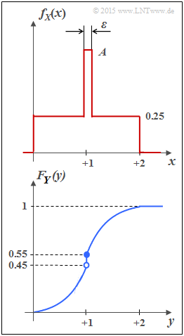
| − | * | + | *For example, the random variable $Y$ with [[Theory_of_Stochastic_Signals/Cumulative_Distribution_Function_(CDF)|cumulative distribution function]] $F_Y(y)$ as shown in the sketch below has both a continuous and a discrete component. |
| − | * | + | *The [[Theory_of_Stochastic_Signals/Wahrscheinlichkeitsdichtefunktion|probability density function]] $f_Y(y)$ is obtained from $F_Y(y)$ by differentiation. |
| − | * | + | *The jump at $y= 1$ in the CDF thus becomes a "Dirac" in the probability density function. |
| − | *In | + | *In subtask '''(4)''' the differential entropy $h(Y)$ of $Y$ is to be determined (in bit), assuming the following equation: |
:$$h(Y) = | :$$h(Y) = | ||
| − | \hspace{0.1cm} - \hspace{-0.45cm} \int\limits_{{\rm supp}\hspace{0.03cm}(\hspace{-0.03cm}f_Y)} \hspace{-0.35cm} f_Y(y) \cdot {\rm log}_2 \hspace{0.1cm} [ f_Y(y) ] \hspace{0.1cm}{\rm d}y | + | \hspace{0.1cm} - \hspace{-0.45cm} \int\limits_{{\rm supp}\hspace{0.03cm}(\hspace{-0.03cm}f_Y)} \hspace{-0.35cm} f_Y(y) \cdot {\rm log}_2 \hspace{0.1cm} \big[ f_Y(y) \big] \hspace{0.1cm}{\rm d}y |
\hspace{0.05cm}.$$ | \hspace{0.05cm}.$$ | ||
| − | *In | + | *In subtask '''(2)''', calculate the differential entropy $h(X)$ of the random variable $X$ whose PDF $f_X(x)$ is sketched above. If one performs a suitable boundary transition, the random variable $X$ also becomes a mixed random variable. |
| − | |||
| − | |||
| − | |||
| − | |||
| − | === | + | Hints: |
| + | *The exercise belongs to the chapter [[Information_Theory/Differentielle_Entropie|Differential Entropy]]. | ||
| + | *Further information on mixed random variables can be found in the chapter [[Theory_of_Stochastic_Signals/Cumulative_Distribution_Function_(CDF)|Cumulative Distribution Function]] of the book "Theory of Stochastic Signals". | ||
| + | |||
| + | |||
| + | |||
| + | |||
| + | ===Questions=== | ||
<quiz display=simple> | <quiz display=simple> | ||
| − | { | + | {What is the PDF height $A$ of $f_X(x)$ around $x = 1$? |
|type="[]"} | |type="[]"} | ||
- $A = 0.5/\varepsilon$, | - $A = 0.5/\varepsilon$, | ||
| Line 34: | Line 37: | ||
- $A = 1/\varepsilon$. | - $A = 1/\varepsilon$. | ||
| − | { | + | {Calculate the differential entropy for different $\varepsilon$–values. |
|type="{}"} | |type="{}"} | ||
$ε = 10^{-1}\text{:} \ \ h(X) \ = \ $ { 0.644 3% } $\ \rm bit$ | $ε = 10^{-1}\text{:} \ \ h(X) \ = \ $ { 0.644 3% } $\ \rm bit$ | ||
| Line 40: | Line 43: | ||
$ε = 10^{-3}\text{:} \ \ h(X) \ = \ $ { -7.2--6.8 } $\ \rm bit$ | $ε = 10^{-3}\text{:} \ \ h(X) \ = \ $ { -7.2--6.8 } $\ \rm bit$ | ||
| − | { | + | {What is the result of the limit $ε \to 0$? |
|type="[]"} | |type="[]"} | ||
| − | + $f_X(x)$ | + | + $f_X(x)$ now has a continuous and a discrete component. |
| − | + | + | + The differential energy $h(X)$ is negative. |
| − | + | + | + The magnitude $|h(X)|$ is infinite. |
| − | { | + | {Which statements are true for the random variable $Y$? |
|type="[]"} | |type="[]"} | ||
| − | - | + | - The CDF value at the point $y = 1$ is $0.5$. |
| − | + $Y$ | + | + $Y$ contains a discrete and a continuous component. |
| − | + | + | + The discrete component at $Y = 1$ occurs with $10\%$ probability. |
| − | - | + | - The continuous component of $Y$ is uniformly distributed. |
| − | + | + | + The differential entropies of $X$ and $Y$ are equal. |
| Line 59: | Line 62: | ||
</quiz> | </quiz> | ||
| − | === | + | ===Solution=== |
{{ML-Kopf}} | {{ML-Kopf}} | ||
| − | '''(1)''' | + | '''(1)''' <u>Proposed solution 2</u> is correct because the integral $1$ over the PDF must yield: |
:$$f_X(x) \hspace{0.1cm}{\rm d}x = | :$$f_X(x) \hspace{0.1cm}{\rm d}x = | ||
0.25 \cdot 2 + (A - 0.25) \cdot \varepsilon \stackrel{!}{=} 1 \hspace{0.3cm} | 0.25 \cdot 2 + (A - 0.25) \cdot \varepsilon \stackrel{!}{=} 1 \hspace{0.3cm} | ||
| Line 67: | Line 70: | ||
\hspace{0.3cm}\Rightarrow\hspace{0.3cm} A = 0.5/\varepsilon +0.25\hspace{0.05cm}.$$ | \hspace{0.3cm}\Rightarrow\hspace{0.3cm} A = 0.5/\varepsilon +0.25\hspace{0.05cm}.$$ | ||
| − | '''(2)''' | + | |
| + | |||
| + | '''(2)''' The differential entropy (in "bit") is given as follows: | ||
:$$h(X) = | :$$h(X) = | ||
\hspace{0.1cm} \hspace{-0.45cm} \int\limits_{{\rm supp}(f_X)} \hspace{-0.35cm} f_X(x) \cdot {\rm log}_2 \hspace{0.1cm} \frac{1}{f_X(x)} \hspace{0.1cm}{\rm d}x | \hspace{0.1cm} \hspace{-0.45cm} \int\limits_{{\rm supp}(f_X)} \hspace{-0.35cm} f_X(x) \cdot {\rm log}_2 \hspace{0.1cm} \frac{1}{f_X(x)} \hspace{0.1cm}{\rm d}x | ||
\hspace{0.05cm}.$$ | \hspace{0.05cm}.$$ | ||
| − | + | We now divide the integral into three partial integrals: | |
:$$h(X) = | :$$h(X) = | ||
\hspace{-0.25cm} \int\limits_{0}^{1-\varepsilon/2} \hspace{-0.15cm} 0.25 \cdot {\rm log}_2 \hspace{0.1cm} \frac{1}{0.25} \hspace{0.1cm}{\rm d}x + | \hspace{-0.25cm} \int\limits_{0}^{1-\varepsilon/2} \hspace{-0.15cm} 0.25 \cdot {\rm log}_2 \hspace{0.1cm} \frac{1}{0.25} \hspace{0.1cm}{\rm d}x + | ||
\hspace{-0.25cm}\int\limits_{1+\varepsilon/2}^{2} \hspace{-0.15cm} 0.25 \cdot {\rm log}_2 \hspace{0.1cm} \frac{1}{0.25} \hspace{0.1cm}{\rm d}x | \hspace{-0.25cm}\int\limits_{1+\varepsilon/2}^{2} \hspace{-0.15cm} 0.25 \cdot {\rm log}_2 \hspace{0.1cm} \frac{1}{0.25} \hspace{0.1cm}{\rm d}x | ||
| − | + \hspace{-0.25cm}\int\limits_{1-\varepsilon/2}^{1+\varepsilon/2} \hspace{-0.15cm} [0.5/\varepsilon + 0.25] \cdot {\rm log}_2 \hspace{0.1cm} \frac{1}{0.5/\varepsilon + 0.25} \hspace{0.1cm}{\rm d}x $$ | + | + \hspace{-0.25cm}\int\limits_{1-\varepsilon/2}^{1+\varepsilon/2} \hspace{-0.15cm} \big [0.5/\varepsilon + 0.25 \big ] \cdot {\rm log}_2 \hspace{0.1cm} \frac{1}{0.5/\varepsilon + 0.25} \hspace{0.1cm}{\rm d}x $$ |
:$$ \Rightarrow \hspace{0.3cm} h(X) = 2 \cdot 0.25 \cdot 2 \cdot (2-\varepsilon) - (0.5 + 0.25 \cdot \varepsilon) \cdot {\rm log}_2 \hspace{0.1cm}(0.5/\varepsilon +0.25) | :$$ \Rightarrow \hspace{0.3cm} h(X) = 2 \cdot 0.25 \cdot 2 \cdot (2-\varepsilon) - (0.5 + 0.25 \cdot \varepsilon) \cdot {\rm log}_2 \hspace{0.1cm}(0.5/\varepsilon +0.25) | ||
\hspace{0.05cm}.$$ | \hspace{0.05cm}.$$ | ||
| − | + | In particular, one obtains | |
| − | * | + | * for $\varepsilon = 0.1$: |
:$$h(X) =1.9 - 0.525 \cdot {\rm log}_2 \hspace{0.1cm}(5.25) = 1.9 - 1.256 | :$$h(X) =1.9 - 0.525 \cdot {\rm log}_2 \hspace{0.1cm}(5.25) = 1.9 - 1.256 | ||
\hspace{0.15cm}\underline{= 0.644\,{\rm bit}} | \hspace{0.15cm}\underline{= 0.644\,{\rm bit}} | ||
\hspace{0.05cm},$$ | \hspace{0.05cm},$$ | ||
| − | * | + | * for $\varepsilon = 0.01$: |
:$$h(X) =1.99 - 0.5025 \cdot {\rm log}_2 \hspace{0.1cm}(50.25)= 1.99 - 2.84 | :$$h(X) =1.99 - 0.5025 \cdot {\rm log}_2 \hspace{0.1cm}(50.25)= 1.99 - 2.84 | ||
\hspace{0.15cm}\underline{= -0.850\,{\rm bit}} | \hspace{0.15cm}\underline{= -0.850\,{\rm bit}} | ||
\hspace{0.05cm}$$ | \hspace{0.05cm}$$ | ||
| − | * | + | * for $\varepsilon = 0.001$: |
:$$h(X) =1.999 - 0.50025 \cdot {\rm log}_2 \hspace{0.1cm}(500.25) = 1.999 - 8.967 | :$$h(X) =1.999 - 0.50025 \cdot {\rm log}_2 \hspace{0.1cm}(500.25) = 1.999 - 8.967 | ||
\hspace{0.15cm}\underline{= -6.968\,{\rm bit}} | \hspace{0.15cm}\underline{= -6.968\,{\rm bit}} | ||
\hspace{0.05cm}.$$ | \hspace{0.05cm}.$$ | ||
| − | '''(3)''' <u> | + | |
| − | * | + | '''(3)''' <u>All the proposed solutions</u> $1$ are correct: |
| − | :$$h(X) = \lim\limits_{\varepsilon \hspace{0.05cm}\rightarrow \hspace{0.05cm} 0} \hspace{0.1cm}[(2-\varepsilon) - (0.5 + 0.25 \cdot \varepsilon) \cdot {\rm log}_2 \hspace{0.1cm}(0.5/\varepsilon +0.25)] | + | *After the boundary transition $\varepsilon → 0$ we obtain for the differential entropy |
| + | :$$h(X) = \lim\limits_{\varepsilon \hspace{0.05cm}\rightarrow \hspace{0.05cm} 0} \hspace{0.1cm}\big[(2-\varepsilon) - (0.5 + 0.25 \cdot \varepsilon) \cdot {\rm log}_2 \hspace{0.1cm}(0.5/\varepsilon +0.25)\big] | ||
= 2\,{\rm bit} - 0.5 \cdot \lim\limits_{\varepsilon \hspace{0.05cm}\rightarrow \hspace{0.05cm} 0}\hspace{0.1cm}{\rm log}_2 \hspace{0.1cm}(0.5/\varepsilon) | = 2\,{\rm bit} - 0.5 \cdot \lim\limits_{\varepsilon \hspace{0.05cm}\rightarrow \hspace{0.05cm} 0}\hspace{0.1cm}{\rm log}_2 \hspace{0.1cm}(0.5/\varepsilon) | ||
\hspace{0.3cm}\Rightarrow\hspace{0.3cm} - \infty | \hspace{0.3cm}\Rightarrow\hspace{0.3cm} - \infty | ||
\hspace{0.05cm}.$$ | \hspace{0.05cm}.$$ | ||
| − | * | + | [[File:P_ID2871__Inf_Z_4_2c_neu.png|right|frame|PDF and CDF of the mixed random variable $X$]] |
| + | *The probability density function (PDF) in this case is given by. | ||
:$$f_X(x) = \left\{ \begin{array}{c} 0.25 + 0.5 \cdot \delta (x-1) \\ 0 \\ \end{array} \right. \begin{array}{*{20}c} {\rm{f\ddot{u}r}} \hspace{0.1cm} 0 \le x \le 2, \\ {\rm sonst} \\ \end{array} | :$$f_X(x) = \left\{ \begin{array}{c} 0.25 + 0.5 \cdot \delta (x-1) \\ 0 \\ \end{array} \right. \begin{array}{*{20}c} {\rm{f\ddot{u}r}} \hspace{0.1cm} 0 \le x \le 2, \\ {\rm sonst} \\ \end{array} | ||
\hspace{0.05cm}.$$ | \hspace{0.05cm}.$$ | ||
| − | + | Consequently, it is a "mixed" random variable with | |
| − | * | + | * a stochastic, uniformly distributed part in the range $0 \le x \le 2$, and |
| − | * | + | * a discrete component at $x = 1$ with probability $0.5$. |
| − | |||
| − | |||
| − | |||
| − | |||
| − | |||
| − | |||
| − | |||
| − | |||
| − | |||
| − | + | The graph shows the PDF $f_X(x)$ on the left and the CDF $F_X(x)$ on the right. | |
| − | <br> | + | <br clear=all> |
| + | '''(4)''' <u>The correct solutions are 2, 3 and 5</u>. | ||
| + | The lower graph shows the PDF and the CDF of the random variable $Y$. You can see: | ||
| + | [[File:P_ID2872__Inf_Z_4_2d_neu.png|right|frame|PDF and CDF of the mixed random variable $Y$]] | ||
| + | * Like $X$ , $Y$ contains a continuous and a discrete part. | ||
| + | * The discrete part occurs with probability ${\rm Pr}(Y = 1) = 0.1$. | ||
| + | * Since $F_Y(y)= {\rm Pr}(Y \le y)$ holds, the right-hand side limit is: | ||
| + | :$$F_Y(y = 1) = 0.55.$$ | ||
| + | * The continuous component is not uniformly distributed; rather, there is a triangular PDF. | ||
| + | *The last proposition is also correct: $h(Y) = h(X) = - \infty$. | ||
| + | <br clear=all> | ||
| + | Because: '''For every random quantity with a discrete part – and it is also extremely small, the differential entropy is equal minus infinity.'''. | ||
{{ML-Fuß}} | {{ML-Fuß}} | ||
| Line 123: | Line 132: | ||
| − | [[Category: | + | [[Category:Information Theory: Exercises|^4.1 Differential Entropy^]] |
Latest revision as of 15:57, 1 October 2021
One speaks of a "mixed random variable", if the random variable contains discrete components in addition to a continuous component.
- For example, the random variable $Y$ with cumulative distribution function $F_Y(y)$ as shown in the sketch below has both a continuous and a discrete component.
- The probability density function $f_Y(y)$ is obtained from $F_Y(y)$ by differentiation.
- The jump at $y= 1$ in the CDF thus becomes a "Dirac" in the probability density function.
- In subtask (4) the differential entropy $h(Y)$ of $Y$ is to be determined (in bit), assuming the following equation:
- $$h(Y) = \hspace{0.1cm} - \hspace{-0.45cm} \int\limits_{{\rm supp}\hspace{0.03cm}(\hspace{-0.03cm}f_Y)} \hspace{-0.35cm} f_Y(y) \cdot {\rm log}_2 \hspace{0.1cm} \big[ f_Y(y) \big] \hspace{0.1cm}{\rm d}y \hspace{0.05cm}.$$
- In subtask (2), calculate the differential entropy $h(X)$ of the random variable $X$ whose PDF $f_X(x)$ is sketched above. If one performs a suitable boundary transition, the random variable $X$ also becomes a mixed random variable.
Hints:
- The exercise belongs to the chapter Differential Entropy.
- Further information on mixed random variables can be found in the chapter Cumulative Distribution Function of the book "Theory of Stochastic Signals".
Questions
Solution
- $$f_X(x) \hspace{0.1cm}{\rm d}x = 0.25 \cdot 2 + (A - 0.25) \cdot \varepsilon \stackrel{!}{=} 1 \hspace{0.3cm} \Rightarrow\hspace{0.3cm}(A - 0.25) \cdot \varepsilon \stackrel{!}{=} 0.5 \hspace{0.3cm}\Rightarrow\hspace{0.3cm} A = 0.5/\varepsilon +0.25\hspace{0.05cm}.$$
(2) The differential entropy (in "bit") is given as follows:
- $$h(X) = \hspace{0.1cm} \hspace{-0.45cm} \int\limits_{{\rm supp}(f_X)} \hspace{-0.35cm} f_X(x) \cdot {\rm log}_2 \hspace{0.1cm} \frac{1}{f_X(x)} \hspace{0.1cm}{\rm d}x \hspace{0.05cm}.$$
We now divide the integral into three partial integrals:
- $$h(X) = \hspace{-0.25cm} \int\limits_{0}^{1-\varepsilon/2} \hspace{-0.15cm} 0.25 \cdot {\rm log}_2 \hspace{0.1cm} \frac{1}{0.25} \hspace{0.1cm}{\rm d}x + \hspace{-0.25cm}\int\limits_{1+\varepsilon/2}^{2} \hspace{-0.15cm} 0.25 \cdot {\rm log}_2 \hspace{0.1cm} \frac{1}{0.25} \hspace{0.1cm}{\rm d}x + \hspace{-0.25cm}\int\limits_{1-\varepsilon/2}^{1+\varepsilon/2} \hspace{-0.15cm} \big [0.5/\varepsilon + 0.25 \big ] \cdot {\rm log}_2 \hspace{0.1cm} \frac{1}{0.5/\varepsilon + 0.25} \hspace{0.1cm}{\rm d}x $$
- $$ \Rightarrow \hspace{0.3cm} h(X) = 2 \cdot 0.25 \cdot 2 \cdot (2-\varepsilon) - (0.5 + 0.25 \cdot \varepsilon) \cdot {\rm log}_2 \hspace{0.1cm}(0.5/\varepsilon +0.25) \hspace{0.05cm}.$$
In particular, one obtains
- for $\varepsilon = 0.1$:
- $$h(X) =1.9 - 0.525 \cdot {\rm log}_2 \hspace{0.1cm}(5.25) = 1.9 - 1.256 \hspace{0.15cm}\underline{= 0.644\,{\rm bit}} \hspace{0.05cm},$$
- for $\varepsilon = 0.01$:
- $$h(X) =1.99 - 0.5025 \cdot {\rm log}_2 \hspace{0.1cm}(50.25)= 1.99 - 2.84 \hspace{0.15cm}\underline{= -0.850\,{\rm bit}} \hspace{0.05cm}$$
- for $\varepsilon = 0.001$:
- $$h(X) =1.999 - 0.50025 \cdot {\rm log}_2 \hspace{0.1cm}(500.25) = 1.999 - 8.967 \hspace{0.15cm}\underline{= -6.968\,{\rm bit}} \hspace{0.05cm}.$$
(3) All the proposed solutions $1$ are correct:
- After the boundary transition $\varepsilon → 0$ we obtain for the differential entropy
- $$h(X) = \lim\limits_{\varepsilon \hspace{0.05cm}\rightarrow \hspace{0.05cm} 0} \hspace{0.1cm}\big[(2-\varepsilon) - (0.5 + 0.25 \cdot \varepsilon) \cdot {\rm log}_2 \hspace{0.1cm}(0.5/\varepsilon +0.25)\big] = 2\,{\rm bit} - 0.5 \cdot \lim\limits_{\varepsilon \hspace{0.05cm}\rightarrow \hspace{0.05cm} 0}\hspace{0.1cm}{\rm log}_2 \hspace{0.1cm}(0.5/\varepsilon) \hspace{0.3cm}\Rightarrow\hspace{0.3cm} - \infty \hspace{0.05cm}.$$
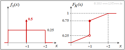
- The probability density function (PDF) in this case is given by.
- $$f_X(x) = \left\{ \begin{array}{c} 0.25 + 0.5 \cdot \delta (x-1) \\ 0 \\ \end{array} \right. \begin{array}{*{20}c} {\rm{f\ddot{u}r}} \hspace{0.1cm} 0 \le x \le 2, \\ {\rm sonst} \\ \end{array} \hspace{0.05cm}.$$
Consequently, it is a "mixed" random variable with
- a stochastic, uniformly distributed part in the range $0 \le x \le 2$, and
- a discrete component at $x = 1$ with probability $0.5$.
The graph shows the PDF $f_X(x)$ on the left and the CDF $F_X(x)$ on the right.
(4) The correct solutions are 2, 3 and 5.
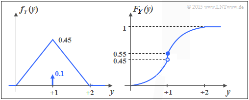
The lower graph shows the PDF and the CDF of the random variable $Y$. You can see:
- Like $X$ , $Y$ contains a continuous and a discrete part.
- The discrete part occurs with probability ${\rm Pr}(Y = 1) = 0.1$.
- Since $F_Y(y)= {\rm Pr}(Y \le y)$ holds, the right-hand side limit is:
- $$F_Y(y = 1) = 0.55.$$
- The continuous component is not uniformly distributed; rather, there is a triangular PDF.
- The last proposition is also correct: $h(Y) = h(X) = - \infty$.
Because: For every random quantity with a discrete part – and it is also extremely small, the differential entropy is equal minus infinity..


