Difference between revisions of "Aufgaben:Exercise 4.1: PDF, CDF and Probability"
m (Text replacement - "value-discrete" to "discrete") |
|||
| (2 intermediate revisions by 2 users not shown) | |||
| Line 1: | Line 1: | ||
| − | {{quiz-Header|Buchseite= | + | {{quiz-Header|Buchseite=Information_Theory/Differential_Entropy |
}} | }} | ||
| Line 9: | Line 9: | ||
| − | The upper plot shows the cumulative distribution function $F_X(x)$ of a | + | The upper plot shows the cumulative distribution function $F_X(x)$ of a discrete random variable $X$. The corresponding probability density function $f_X(x)$ has to be determined in subtask '''(1)'''. |
The equation | The equation | ||
| Line 19: | Line 19: | ||
:$$ f_Y(y) = \left\{ \begin{array}{c} \hspace{0.1cm}1/2 \cdot \cos^2(\pi/4 \cdot y) \\ \hspace{0.1cm} 0 \\ \end{array} \right.\quad \begin{array}{*{20}c} {\rm{f\ddot{u}r}} \\ {\rm{f\ddot{u}r}} \\ \end{array}\begin{array}{*{20}l} | y| \le 2, \\ | :$$ f_Y(y) = \left\{ \begin{array}{c} \hspace{0.1cm}1/2 \cdot \cos^2(\pi/4 \cdot y) \\ \hspace{0.1cm} 0 \\ \end{array} \right.\quad \begin{array}{*{20}c} {\rm{f\ddot{u}r}} \\ {\rm{f\ddot{u}r}} \\ \end{array}\begin{array}{*{20}l} | y| \le 2, \\ | ||
y < -2 \hspace{0.1cm}{\rm und}\hspace{0.1cm}y > +2 \\ \end{array}$$ | y < -2 \hspace{0.1cm}{\rm und}\hspace{0.1cm}y > +2 \\ \end{array}$$ | ||
| − | of a | + | of a continuous random variable $Y$, which is restricted to the range $|Y| \le 2$ . |
| − | In principle, the same relationship between PDF, CDF and probabilities exists for the | + | In principle, the same relationship between PDF, CDF and probabilities exists for the continuous random variable $Y$ as for a discrete random variable. Nevertheless, you will notice some differences in details. |
| − | For example, for the | + | For example, for the continuous random variable $Y$, the boundary transition can be omitted in the above equation, and we obtain simplified: |
:$${\rm Pr}(A \le Y \le B) = F_Y(B) - F_Y(A) =\int_{A}^{B} \hspace{-0.01cm} f_Y(y) | :$${\rm Pr}(A \le Y \le B) = F_Y(B) - F_Y(A) =\int_{A}^{B} \hspace{-0.01cm} f_Y(y) | ||
\hspace{0.1cm}{\rm d}y\hspace{0.05cm}.$$ | \hspace{0.1cm}{\rm d}y\hspace{0.05cm}.$$ | ||
| Line 36: | Line 36: | ||
Hints: | Hints: | ||
*The exercise belongs to the chapter [[Information_Theory/Differentielle_Entropie|Differential Entropy]]. | *The exercise belongs to the chapter [[Information_Theory/Differentielle_Entropie|Differential Entropy]]. | ||
| − | *Useful hints for solving this problem and further information on | + | *Useful hints for solving this problem and further information on continuous random variables can be found in the third chapter "Continuous Random Variables" of the book [[Theory of Stochastic Signals]]. |
*Given also is the following indefinite integral: | *Given also is the following indefinite integral: | ||
| Line 46: | Line 46: | ||
<quiz display=simple> | <quiz display=simple> | ||
| − | {Determine the PDF $f_X(x)$ of the | + | {Determine the PDF $f_X(x)$ of the discrete random variable $X$. Which of the following statements are true? |
|type="[]"} | |type="[]"} | ||
+ The PDF is composed of five Dirac functions. | + The PDF is composed of five Dirac functions. | ||
| Line 58: | Line 58: | ||
${\rm Pr}(|X| ≤ 1) \ = \ $ { 0.8 3% } | ${\rm Pr}(|X| ≤ 1) \ = \ $ { 0.8 3% } | ||
| − | {What are the values of the cumulative distribution function $F_Y(y) ={\rm Pr}(Y \le y)$ of the | + | {What are the values of the cumulative distribution function $F_Y(y) ={\rm Pr}(Y \le y)$ of the continuous random variable $Y$, in particular: |
|type="{}"} | |type="{}"} | ||
$F_Y(y = 0) \ = \ $ { 0.5 3% } | $F_Y(y = 0) \ = \ $ { 0.5 3% } | ||
| Line 81: | Line 81: | ||
===Solution=== | ===Solution=== | ||
{{ML-Kopf}} | {{ML-Kopf}} | ||
| − | [[File:P_ID2857__Inf_A_4_1a_neu.png|right|frame|PDF and CDF of the | + | [[File:P_ID2857__Inf_A_4_1a_neu.png|right|frame|PDF and CDF of the discrete random variable $X$]] |
'''(1)''' <u>Proposed solutions 1 and 2</u> are correct: | '''(1)''' <u>Proposed solutions 1 and 2</u> are correct: | ||
*The cumulative distribution function $F_X(x)$ is obtained from the probability density function $f_X(x)$ by integration over the (renamed) random variable in the range from $- \infty$ to $x$. | *The cumulative distribution function $F_X(x)$ is obtained from the probability density function $f_X(x)$ by integration over the (renamed) random variable in the range from $- \infty$ to $x$. | ||
| Line 105: | Line 105: | ||
\hspace{0.15cm}\underline {= 0.8}\hspace{0.05cm}.$$ | \hspace{0.15cm}\underline {= 0.8}\hspace{0.05cm}.$$ | ||
| − | The same result is obtained using the CDF. Here the general equation, which is equally valid for | + | The same result is obtained using the CDF. Here the general equation, which is equally valid for discrete and continuous random variables, is: |
:$${\rm Pr}(A < X \le B) =F_X(B) - F_X(A) \hspace{0.05cm}.$$ | :$${\rm Pr}(A < X \le B) =F_X(B) - F_X(A) \hspace{0.05cm}.$$ | ||
| Line 115: | Line 115: | ||
| − | [[File:P_ID2858__Inf_A_4_1c_neu.png|right|frame|PDF and CDF of the | + | [[File:P_ID2858__Inf_A_4_1c_neu.png|right|frame|PDF and CDF of the continuous random variable $Y$]] |
'''(3)''' The cumulative distribution function $F_Y(y)$ is obtained from the (renamed) WDF $f_Y(\eta)$ by integrating $- \infty$ to $x$. Due to symmetry, this can be written in the range $0 \le y \le +2$: | '''(3)''' The cumulative distribution function $F_Y(y)$ is obtained from the (renamed) WDF $f_Y(\eta)$ by integrating $- \infty$ to $x$. Due to symmetry, this can be written in the range $0 \le y \le +2$: | ||
:$$F_Y(y) = \int_{-\infty}^{\hspace{0.05cm}y} \hspace{-0.1cm}f_Y(\eta) \hspace{0.1cm}{\rm d}\eta ={1}/{2}+\int_{0}^{\hspace{0.05cm}y} \hspace{-0.1cm}f_Y(\eta) \hspace{0.1cm}{\rm d}\eta$$ | :$$F_Y(y) = \int_{-\infty}^{\hspace{0.05cm}y} \hspace{-0.1cm}f_Y(\eta) \hspace{0.1cm}{\rm d}\eta ={1}/{2}+\int_{0}^{\hspace{0.05cm}y} \hspace{-0.1cm}f_Y(\eta) \hspace{0.1cm}{\rm d}\eta$$ | ||
| Line 126: | Line 126: | ||
| − | '''(4)''' The probability that the | + | '''(4)''' The probability that the continuous random variable $Y$ lies in the range from $-\varepsilon$ to $+\varepsilon$ can be calculated using the given equation as follows: |
:$${\rm Pr}(-\varepsilon \le Y \le +\varepsilon) = F_Y(+\varepsilon) - F_Y(-\varepsilon) \hspace{0.05cm}.$$ | :$${\rm Pr}(-\varepsilon \le Y \le +\varepsilon) = F_Y(+\varepsilon) - F_Y(-\varepsilon) \hspace{0.05cm}.$$ | ||
| Line 135: | Line 135: | ||
F_Y(y \hspace{0.05cm}\rightarrow\hspace{0.05cm}0^{+}) - F_Y(y \hspace{0.05cm}\rightarrow\hspace{0.05cm}0^{-})\hspace{0.05cm}.$$ | F_Y(y \hspace{0.05cm}\rightarrow\hspace{0.05cm}0^{+}) - F_Y(y \hspace{0.05cm}\rightarrow\hspace{0.05cm}0^{-})\hspace{0.05cm}.$$ | ||
| − | *Since for a | + | *Since for a continuous random variable the two limits are equal, $\underline{{\rm Pr}(Y = 0) = 0}$. |
| − | '''In general''': The probability ${\rm Pr}(Y = y_0)$ that a | + | '''In general''': The probability ${\rm Pr}(Y = y_0)$ that a continuous random variable $Y$ takes a fixed value $y_0$, is always zero. |
| Line 149: | Line 149: | ||
| − | '''(6)''' We again assume the equation $ {\rm Pr}(A \le Y \le B) = F_Y(B) - F_Y(A)$ valid for the | + | '''(6)''' We again assume the equation $ {\rm Pr}(A \le Y \le B) = F_Y(B) - F_Y(A)$ valid for the continuous random quantity $Y$: |
*With $A = 0$ and $B \to \infty$ $($or $B = 2)$ we obtain: | *With $A = 0$ and $B \to \infty$ $($or $B = 2)$ we obtain: | ||
:$${\rm Pr}( Y > 0) = {\rm Pr}(0 \le Y \le \infty) | :$${\rm Pr}( Y > 0) = {\rm Pr}(0 \le Y \le \infty) | ||
| Line 155: | Line 155: | ||
\hspace{0.15cm}\underline {= 0.5}\hspace{0.05cm}.$$ | \hspace{0.15cm}\underline {= 0.5}\hspace{0.05cm}.$$ | ||
*Thus, for the symmetric continuous random variable $Y$ holds indeed as expected: ${\rm Pr}( Y > 0) = 1/2$. | *Thus, for the symmetric continuous random variable $Y$ holds indeed as expected: ${\rm Pr}( Y > 0) = 1/2$. | ||
| − | *Although the | + | *Although the discrete random variable $X$ is also symmetrical about $x= 0$ ⇒ ${\rm Pr}( X > 0) = 0.3$ was determined in subtask '''(3)''', on the other hand. |
*Further, with $A = -1$ and $B = +1$, one obtains because of $F_Y(-1) = 1- F_Y(+1)$: | *Further, with $A = -1$ and $B = +1$, one obtains because of $F_Y(-1) = 1- F_Y(+1)$: | ||
:$${\rm Pr}( |Y| \le 1) = {\rm Pr}(-1 \le Y \le +1) | :$${\rm Pr}( |Y| \le 1) = {\rm Pr}(-1 \le Y \le +1) | ||
Latest revision as of 10:27, 11 October 2021
To repeat some important basics from the book "Theory of Stochastic Signals" we are dealing with
- the probability density function $\rm (PDF)$,
- the cumulative distribution function $\rm (CDF)$.
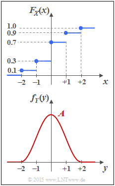
The upper plot shows the cumulative distribution function $F_X(x)$ of a discrete random variable $X$. The corresponding probability density function $f_X(x)$ has to be determined in subtask (1).
The equation
- $$ {\rm Pr}(A < X \le B) = F_X(B) - F_X(A) = \lim_{\varepsilon \hspace{0.05cm}\rightarrow \hspace{0.05cm}0} \int_{A+\varepsilon}^{B+\varepsilon} \hspace{-0.15cm} f_X(x) \hspace{0.1cm}{\rm d}x $$
represents two ways to calculate the probability for the event "The random variable $X$ lies in a given interval" from the CDF and the PDF, respectively.
The lower graph shows the probability density function
- $$ f_Y(y) = \left\{ \begin{array}{c} \hspace{0.1cm}1/2 \cdot \cos^2(\pi/4 \cdot y) \\ \hspace{0.1cm} 0 \\ \end{array} \right.\quad \begin{array}{*{20}c} {\rm{f\ddot{u}r}} \\ {\rm{f\ddot{u}r}} \\ \end{array}\begin{array}{*{20}l} | y| \le 2, \\ y < -2 \hspace{0.1cm}{\rm und}\hspace{0.1cm}y > +2 \\ \end{array}$$
of a continuous random variable $Y$, which is restricted to the range $|Y| \le 2$ . In principle, the same relationship between PDF, CDF and probabilities exists for the continuous random variable $Y$ as for a discrete random variable. Nevertheless, you will notice some differences in details.
For example, for the continuous random variable $Y$, the boundary transition can be omitted in the above equation, and we obtain simplified:
- $${\rm Pr}(A \le Y \le B) = F_Y(B) - F_Y(A) =\int_{A}^{B} \hspace{-0.01cm} f_Y(y) \hspace{0.1cm}{\rm d}y\hspace{0.05cm}.$$
Hints:
- The exercise belongs to the chapter Differential Entropy.
- Useful hints for solving this problem and further information on continuous random variables can be found in the third chapter "Continuous Random Variables" of the book Theory of Stochastic Signals.
- Given also is the following indefinite integral:
- $$\int \hspace{0.1cm} \cos^2(A \eta) \hspace{0.1cm}{\rm d}\eta = \frac{\eta}{2} + \frac{1}{4A} \cdot \sin(2A \eta).$$
Questions
Solution
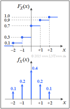
(1) Proposed solutions 1 and 2 are correct:
- The cumulative distribution function $F_X(x)$ is obtained from the probability density function $f_X(x)$ by integration over the (renamed) random variable in the range from $- \infty$ to $x$.
- The inverse is: Given the CDF, obtain the PDF by differentiation.
- The given CDF contains five discontinuity points, which after differentiation lead to five Dirac functions:
- $$f_X(x) = 0.1 \cdot {\rm \delta}( x+2) + 0.2 \cdot {\rm \delta}( x+1) + 0.4 \cdot {\rm \delta}( x) + 0.2 \cdot {\rm \delta}( x-1) + 0.1 \cdot {\rm \delta}( x-2)\hspace{0.05cm}.$$
- The Dirac weights give the occurrence probabilities of the random variable $X = \{-2,\ -1,\ 0,\ +1,\ +2\}$ , e.g.:
- $${\rm Pr}(X = 0) = F_X(x \hspace{0.05cm}\rightarrow\hspace{0.05cm}0^{+}) - F_X(x \hspace{0.05cm}\rightarrow\hspace{0.05cm}0^{-}) = 0.7 - 0.3 = 0.4\hspace{0.05cm}.$$
- Accordingly, the other probabilities are:
- $${\rm Pr}(X = +1) = {\rm Pr}(X = -1) = 0.2\hspace{0.05cm},\hspace{0.3cm} {\rm Pr}(X = +2) = {\rm Pr}(X = -2) = 0.1\hspace{0.05cm}.$$
(2) From the PDF just calculated, we obtain:
- $${\rm Pr}(X >0) = {\rm Pr}(X = +1) + {\rm Pr}(X = +2) \hspace{0.15cm}\underline {= 0.3}\hspace{0.05cm},$$
- $${\rm Pr}(|X| \le 1) ={\rm Pr}(X = -1) + {\rm Pr}(X = 0) + {\rm Pr}(X = +1) = 0.2 + 0.4 +0.2 \hspace{0.15cm}\underline {= 0.8}\hspace{0.05cm}.$$
The same result is obtained using the CDF. Here the general equation, which is equally valid for discrete and continuous random variables, is:
- $${\rm Pr}(A < X \le B) =F_X(B) - F_X(A) \hspace{0.05cm}.$$
- Thus, with $A= 0$ and $B = +2$ we obtain:
- $${\rm Pr}(0 < X \le +2) = {\rm Pr}(X >0)= F_X(+2) - F_X(0) = 1 - 0.7 \hspace{0.15cm}\underline {= 0.3} \hspace{0.05cm}.$$
- Setting $A=-2$ and $B = +1$, we get:
- $${\rm Pr}(-2 < X \le +1) = {\rm Pr}(|X| \le 1)= F_X(+1) - F_X(-2) = 0.9 - 0.1 \hspace{0.15cm}\underline {= 0.8} \hspace{0.05cm}.$$
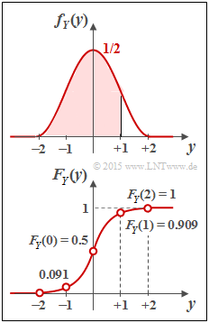
(3) The cumulative distribution function $F_Y(y)$ is obtained from the (renamed) WDF $f_Y(\eta)$ by integrating $- \infty$ to $x$. Due to symmetry, this can be written in the range $0 \le y \le +2$:
- $$F_Y(y) = \int_{-\infty}^{\hspace{0.05cm}y} \hspace{-0.1cm}f_Y(\eta) \hspace{0.1cm}{\rm d}\eta ={1}/{2}+\int_{0}^{\hspace{0.05cm}y} \hspace{-0.1cm}f_Y(\eta) \hspace{0.1cm}{\rm d}\eta$$
- $$\Rightarrow \hspace{0.3cm}F_Y(y) = \frac{1}{2}+\int_{0}^{\hspace{0.05cm}y} \hspace{0.1cm}\frac{1}{2} \cdot \cos^2({\pi}/{4} \cdot \eta) \hspace{0.1cm}{\rm d}\eta = \frac{1}{2}+\frac{y}{4} + \frac{1}{2\pi} \cdot \sin({\pi}/{2} \cdot y).$$
The equation holds in the entire range $0 \le y \le +2$. The CDF values we are looking for are thus:
- $F_Y(y=0)\hspace{0.15cm}\underline{= 0.5}$ (integral over half the PDF),
- $F_Y(y=1)= 3/4 + 1/(2 \pi)\hspace{0.15cm}\underline{= 0.909}$ (area in red background in the PDF),
- $F_Y(y=2)\hspace{0.15cm}\underline{= 1}$ (integral over the entire PDF).
(4) The probability that the continuous random variable $Y$ lies in the range from $-\varepsilon$ to $+\varepsilon$ can be calculated using the given equation as follows:
- $${\rm Pr}(-\varepsilon \le Y \le +\varepsilon) = F_Y(+\varepsilon) - F_Y(-\varepsilon) \hspace{0.05cm}.$$
- It was taken into account that for the random variable $Y$ the "<"sign can be replaced by the "≤" sign without distortion.
- With the boundary transition $\varepsilon \to 0$, the probability we are looking for is obtained:
- $${\rm Pr}(Y = 0) =\lim_{\varepsilon\hspace{0.05cm}\rightarrow\hspace{0.05cm}0}\hspace{0.1cm}{\rm Pr}(-\varepsilon \le Y \le +\varepsilon) = \lim_{\varepsilon\hspace{0.05cm}\rightarrow\hspace{0.05cm}0}\hspace{0.1cm} F_Y(+\varepsilon) - \lim_{\varepsilon\hspace{0.05cm}\rightarrow\hspace{0.05cm}0}\hspace{0.1cm} F_Y(-\varepsilon) = F_Y(y \hspace{0.05cm}\rightarrow\hspace{0.05cm}0^{+}) - F_Y(y \hspace{0.05cm}\rightarrow\hspace{0.05cm}0^{-})\hspace{0.05cm}.$$
- Since for a continuous random variable the two limits are equal, $\underline{{\rm Pr}(Y = 0) = 0}$.
In general: The probability ${\rm Pr}(Y = y_0)$ that a continuous random variable $Y$ takes a fixed value $y_0$, is always zero.
(5) Proposed solution 2 is correct:
- Based on the PDF at hand, the result $Y=3$ can be excluded.
- The result $Y=0$ on the other hand is quite possible, although ${\rm Pr}(Y = 0) = 0$ .
- For example, if one performs a random experiment $N \to \infty$ times and obtains the result $Y= 0$ for $N_0$ times, then with finite $N_0$ according to the classical definition of probability:
- $${\rm Pr}(Y = 0) = \lim_{N\hspace{0.05cm}\rightarrow\hspace{0.05cm}\infty}\hspace{0.1cm}{N_0}/{N} = 0\hspace{0.05cm}.$$
(6) We again assume the equation $ {\rm Pr}(A \le Y \le B) = F_Y(B) - F_Y(A)$ valid for the continuous random quantity $Y$:
- With $A = 0$ and $B \to \infty$ $($or $B = 2)$ we obtain:
- $${\rm Pr}( Y > 0) = {\rm Pr}(0 \le Y \le \infty) = {\rm Pr}(0 \le Y \le 2) = F_Y(2) - F_Y(0) \hspace{0.15cm}\underline {= 0.5}\hspace{0.05cm}.$$
- Thus, for the symmetric continuous random variable $Y$ holds indeed as expected: ${\rm Pr}( Y > 0) = 1/2$.
- Although the discrete random variable $X$ is also symmetrical about $x= 0$ ⇒ ${\rm Pr}( X > 0) = 0.3$ was determined in subtask (3), on the other hand.
- Further, with $A = -1$ and $B = +1$, one obtains because of $F_Y(-1) = 1- F_Y(+1)$:
- $${\rm Pr}( |Y| \le 1) = {\rm Pr}(-1 \le Y \le +1) = F_Y(+1) - F_Y(-1) = 2 \cdot F_Y(+1) -1 = 2 \cdot 0.909 -1 \hspace{0.15cm}\underline {= 0.818}. $$


