Difference between revisions of "Theory of Stochastic Signals/Auto-Correlation Function"
| Line 189: | Line 189: | ||
Based on these representations, the following statements are possible: | Based on these representations, the following statements are possible: | ||
*$\{y_i(t)\}$ has stronger internal statistical bindings than $\{x_i(t)\}$. Spectrally, the process $\{y_i(t)\}$ is thus lower frequency. | *$\{y_i(t)\}$ has stronger internal statistical bindings than $\{x_i(t)\}$. Spectrally, the process $\{y_i(t)\}$ is thus lower frequency. | ||
| − | *The sketched pattern signals $x(t)$ and $y(t)$ already suggest that both processes are mean | + | *The sketched pattern signals $x(t)$ and $y(t)$ already suggest that both processes are zero mean and have the same rms value. |
*The above autocorrelation functions confirm these statements. The liear mean values $m_x = m_y = 0$ result in each case from the ACF–limit for $τ → ∞$. | *The above autocorrelation functions confirm these statements. The liear mean values $m_x = m_y = 0$ result in each case from the ACF–limit for $τ → ∞$. | ||
*Because $m_x = 0$ applies here to the variance: $σ_x^2 = φ_x(0) = 0.01 \hspace{0.05cm} \rm V^2$, and the rms value is consequently $σ_x = 0.1 \hspace{0.05cm}\rm V$. | *Because $m_x = 0$ applies here to the variance: $σ_x^2 = φ_x(0) = 0.01 \hspace{0.05cm} \rm V^2$, and the rms value is consequently $σ_x = 0.1 \hspace{0.05cm}\rm V$. | ||
| Line 234: | Line 234: | ||
$\text{Conclusion:}$ | $\text{Conclusion:}$ | ||
*If the signal values are only available at discrete time points $($at multiples of $T_{\rm A})$ , one can also determine the autocorrelation function only at integer multiples of $T_{\rm A}$ . | *If the signal values are only available at discrete time points $($at multiples of $T_{\rm A})$ , one can also determine the autocorrelation function only at integer multiples of $T_{\rm A}$ . | ||
| − | *With the discrete-time signal values $x_ν = x(ν - T_{\rm A})$ and $x_{ν+k} = x((ν+k) - T_{\rm A})$ and the discrete-time ACF $φ_k = φ_x(k - T_{\rm A})$ the | + | *With the discrete-time signal values $x_ν = x(ν - T_{\rm A})$ and $x_{ν+k} = x((ν+k) - T_{\rm A})$ and the discrete-time ACF $φ_k = φ_x(k - T_{\rm A})$ the ACF calculation can thus be represented as follows: |
:$$\varphi_k = \overline {x_\nu \cdot x_{\nu + k} }.$$ | :$$\varphi_k = \overline {x_\nu \cdot x_{\nu + k} }.$$ | ||
The sweeping line again denotes time averaging}}. | The sweeping line again denotes time averaging}}. | ||
| Line 256: | Line 256: | ||
$\text{Conclusion:}$ | $\text{Conclusion:}$ | ||
Following this scheme results in the following algorithm: | Following this scheme results in the following algorithm: | ||
| − | *You define the field $\rm | + | *You define the field $\rm ACF\big[\hspace{0.05cm}0 : {\it l}\hspace{0.1cm}\big]$ of type "float" and preallocate zeros to all elements. |
*On each loop pass $($indexed with variable $k)$ the $l + 1$ field elements ${\rm ACF}\big[\hspace{0.03cm}k\hspace{0.03cm}\big]$ are incremented by the contribution $x_ν - x_{ν+k}$ respectively. | *On each loop pass $($indexed with variable $k)$ the $l + 1$ field elements ${\rm ACF}\big[\hspace{0.03cm}k\hspace{0.03cm}\big]$ are incremented by the contribution $x_ν - x_{ν+k}$ respectively. | ||
*All $l+1$ field elements are processed, however, only as long as the run variable $k$ is not greater than $N - l$ . | *All $l+1$ field elements are processed, however, only as long as the run variable $k$ is not greater than $N - l$ . | ||
Revision as of 00:30, 28 February 2022
Contents
- 1 Random processes
- 2 Stationary random processes
- 3 Ergodic random processes
- 4 Generally valid description of random processes
- 5 General definition of the autocorrelation function
- 6 ACF for ergodic processes
- 7 Properties of the autocorrelation function
- 8 Interpretation of the autocorrelation function
- 9 Numerical ACF determination
- 10 Genauigkeit der numerischen AKF-Berechnung
- 11 Aufgaben zum Kapitel
Random processes
An important concept in stochastic signal theory is the random process. Below are some characteristics of such a stochastic process - these terms are used synonymously both in the literature and in our tutorial.
$\text{Definitions:}$ By a random process $\{x_i(t)\}$ we understand a mathematical model for an ensemble of (many) random signals, which can and will differ from each other in detail, but nevertheless have certain common properties.
- To describe a random process $\{x_i(t)\}$ we start from the notion that there are any number of random generators, completely identical in their physical and statistical properties, each of which yields a random signal $x_i(t)$ .
- Each random generator, despite having the same physical realization, outputs a different time signal $x_i(t)$ that exists for all times from $-∞$ to $+∞$ This specific random signal is called the $i$-th pattern signal.
- Every random process involves at least one stochastic component - for example, the amplitude, frequency, or phase of a message signal - and therefore cannot be accurately predicted by an observer.
- The random process differs from the usual random experiments in probability or statistics in that the result is not an event but a function (time signal).
- If we consider the random process $\{x_i(t)\}$ at a fixed time, we return to the simpler model from the chapter From Random Experiment to Random Variable, according to which the experimental result is an event that can be assigned to a random variable
.
These statements are now illustrated by the example of a binary random generator, which - at least in thought - can be realized arbitrarily often.
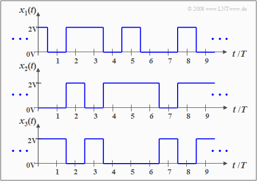
$\text{Example 1:}$ The graph shows three different pattern signals of a random process with the following properties:
- The random process here $\{x_i(t)\}$ consists of an ensemble of rectangular pattern functions, which can be described as follows:
- $$x_i(t)=\sum^{+\infty}_{\nu=-\infty} (a_\nu)_i\cdot g(t-\nu \cdot T ).$$
- The fundamental momentum $g(t)$ has in the range from $-T/2$ to $+T/2$ the value $2\hspace{0.03cm}\rm V$; outside it is zero and exactly at $\pm T/2$ only half as large $(1\hspace{0.03cm}\rm V)$.
- Remember: A pulse, as defined in the chapter Signal Classification in the book "Signal Representation", is both a deterministic and energy-limited signal.
- The statistics of the random process under consideration is due solely to the dimensionless amplitude coefficients $(a_ν)_i ∈ \{0, 1\}$ which are time-indexed $ν$ for the $i$-th pattern function.
- Despite the different signal courses in detail, the sketched signals $x_1(t)$, $x_2(t)$, $x_3(t)$ and also all further pattern signals $x_4(t)$, $x_5(t)$, $x_6(t)$, ... have certain common features, which will be elaborated in the following.
Stationary random processes
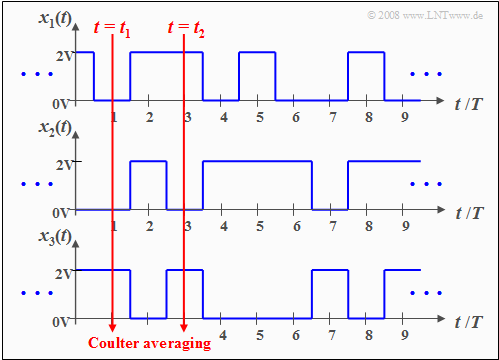
If one defines the instantaneous value of all pattern functions $x_i(t)$ at a fixed time $t = t_1$ as a new random variable $x_1 = \{ x_i(t_1)\}$, its statistical properties can be described according to the statements
- of the second chapter "Discrete Random Variables" and
- of the third chapter "Continuous Random Variables"
in this book.
Similarly, for the time of observation $t = t_2$ we obtain the random variable $x_2 = \{ x_i(t_2)\}$.
Note on nomenclature: Note that.
- $x_1(t)$ and $x_2(t)$ are sample functions of the random process $\{x_i(t)\}$ ,
- while the random variables $x_1$ and $x_2$ characterize the whole process at times $t_1$ and $t_2$ respectively.
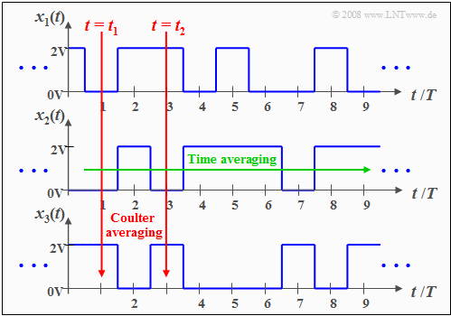
The calculation of the statistical characteristics must be done by coulter averaging over all possible pattern functions $($averaging over the run variable $i$, i.e. over all realizations$)$.
$\text{Definition:}$
- For a stationary random process $\{x_i(t)\}$ all statistical parameters $($mean, standard deviation, higher order moments, probabilities of occurrence, etc. $)$ of the random variables $x_1 = \{ x_i(t_1)\}$ and $x_2 = \{ x_i(t_2)\}$ are equal.
- Also at other times, the values are exactly the same.
The converse is One calls a random process $\{x_i(t)\}$ a non-stationary if it has different statistical properties at different times.
$\text{Example 2:}$ A large number of measuring stations at the equator determine the temperature daily at 12 o'clock local time. If one averages over all these measured values, one can eliminate the influence of local indicators (e.g. Gulf Stream). If one plots the mean values (coulter averaging) over time, almost a constant will result, and one can speak of a stationary process .
A comparable series of measurements at 50° latitude would indicate a non-stationary process due to the seasonal variations, with significant differences in mean and variance of the noon temperature between January and July.
Ergodic random processes
An important subclass of stationary random processes are the so-called ergodic processes with the following properties:
$\text{Definition:}$ In an ergodic process $\{x_i(t)\}$ each individual pattern function $x_i(t)$ is representative of the entire ensemble.
- All statistical descriptive quantities of an ergodic process can be obtained from a single pattern function by time averaging $($referring to the running variables $ν = t/T$ ⇒ normalized time$)$ .
- This also means that With ergodicity, the time averages of each sample function coincide with the corresponding coulter averages at arbitrary time points $ν$.
For example, with ergodicity, for the moment $k$-th order:
- $$m_k=\overline{x^k(t)}={\rm E}\big[x^k\big].$$
Here, the sweeping line denotes the time mean, while the coulter mean is to be determined by expected value generation $\rm E\big[ \hspace{0.1cm}\text{...} \hspace{0.1cm} \big]$ as described in chapter Moments of a discrete random variable .
Note: Ergodicity cannot be proved from a finite number of pattern functions and finite signal sections.
- However, ergodicity is hypothetically - but nevertheless quite justifiably - assumed in most applications.
- On the basis of the results found, the plausibility of this ergodicity hypothesis must subsequently be checked.
Generally valid description of random processes
If the random process to be analyzed $\{x_i(t)\}$ is not stationary and thus certainly not ergodic, the moments must always be determined as coulter averages. In general, these are time-dependent:
- $$m_k(t_1) \ne m_k(t_2).$$
However, since by the moments also the characteristic function (Fourier retransform of the PDF).
- $$ C_x(\Omega) ={\rm\sum^{\infty}_{{\it k}=0}}\ \frac{m_k}{k!}\cdot \Omega^{k}\ \circ\!\!-\!\!\!-\!\!\!-\!\!\bullet\,\ f_{x}(x)$$
is fixed, the probability density function $f_{x}(x)$ is also time dependent.
If not only the amplitude distributions at different times $t_1, t_2$, ... are to be determined, but also the statistical bindings between the signal values at these times, one has to pass to the joint probability density function .
For example, considering the two time points $t_1$ and $t_2$, note the following:
- The 2D PDF is obtained according to the specifications on page properties and examples of two-dimensional random variables with $x = x(t_1)$ and $y = x(t_2)$. It is obvious that already the determination of this quantity is very complex.
- If one further considers that to capture all statistical bindings within the random process actually the $n$-dimensional joint probability density function (joint PDF) would have to be used, where if possible the limit $n → ∞$ still has to be formed, one recognizes the difficulties for the solution of practical problems.
- For these reasons, in order to describe the statistical bindings of a random process, one proceeds to the autocorrelation function, which simplifies the problem. This is first defined in the following section for the general case.
General definition of the autocorrelation function
$\text{General definition:}$ The autocorrelation function (ACF) of a random process $\{x_i(t)\}$ is equal to the expected value of the product of the signal values at two time points $t_1$ and $t_2$:
- $$\varphi_x(t_1,t_2)={\rm E}\big[x(t_{\rm 1})\cdot x(t_{\rm 2})\big].$$
This definition holds whether the random process is ergodic or nonergodic, and it also holds in principle for nonstationary processes.
Note on nomenclature:
In order to establish the relationship with the Cross-Correlation Function $φ_{xy}$ between the two statistical quantities $x$ and $y$ to make clear, in some literature for the autocorrelation function instead of $φ_{x}$ the notation $φ_{xx}$ is also often used. In our learning tutorial, we refrain from doing so.
A comparison with the section Expected values of two-dimensional random variables shows that the ACF–value $φ_x(t_1, t_2)$ indicates the joint moment $m_{11}$ between the two random variables $x(t_1)$ and $x(t_2)$ .
While exact statements regarding the statistical bindings of a random process actually require the $n$–dimensional joint density $($with $n → ∞)$ , the following simplifications are implicitly made by moving to the autocorrelation function:
- Instead of infinitely many time points, only two are considered here, and instead of all moments $m_{\hspace{0.05cm}k\hspace{0.05cm}l}$ at the two time points $t_1$ and $t_2$ with $k, \ l ∈ \{1, 2, 3, \text{...} \}$ only the joint moment $m_{11}$ is captured here.
- The moment $m_{11}$ exclusively reflects the linear dependence ("correlation") of the process. All higher order statistical bindings, on the other hand, are not considered.
- Therefore, when evaluating random processes by means of ACF, it should always be taken into account that it allows only very limited statements about the statistical bindings in general.
$\text{Example 3:}$ The above definition of the autocorrelation function applies in general, i.e. also to non-stationary and non-ergodic processes.
- An example of a non-stationary process is the occurrence of pulse interference in the telephone network caused by dial pulses in adjacent lines.
- In digital signal transmission, such non-stationary interference processes usually lead to trunking errors
.
ACF for ergodic processes
On the autocorrelation function in ergodic processes.
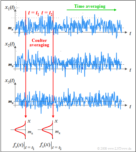
Such a random process $\{x_i(t)\}$ is used as a basis, for example, in the study of Thermal noise . This is based on the notion that
- there are any number of resistors, completely identical in their physical and statistical properties,
- each of which emits a different random signal $x_i(t)$ .
The graph shows such a stationary and ergodic process:
- The individual pattern functions $x_i(t)$ can take on any arbitrary values at any arbitrary times. This means that the random process considered here $\{x_i(t)\}$ is both continuous in value and continuous in time.
- Although no conclusions can be drawn about the actual signal values of the individual pattern functions due to stochasticity, the moments and PDF are the same at all time points.
- In the graph, for reasons of a generalized representation, a DC component $m_x$ is also considered, which, however, is not present in thermal noise.
$\text{Definition:}$ One speaks of a stationary random process $\{x_i(t)\}$ if its statistical properties are invariant to time shifts.
- For the autocorrelation function (ACF), this statement means that it is no longer a function of the two independent time variables $t_1$ and $t_2$ but depends only on the time difference $τ = t_2 - t_1$ :
- $$\varphi_x(t_1,t_2)\rightarrow{\varphi_x(\tau)={\rm E}\big[x(t)\cdot x(t+\tau)\big]}.$$
- The coulter averaging can be done at any time $t$ in this case.
Under the further assumption of an ergodic random process, all moments can also be obtained by time averaging over a single selected pattern function $x(t)$ All these time averages coincide with the corresponding coulter averages in this special case.
$\text{Definition:}$ Thus, for the ACF of an ergodic random process whose pattern signals each range from $-∞$ to $+∞$ $(T_{\rm M}$ denotes the measurement duration$)$ follows:
- $$\varphi_x(\tau)=\overline{x(t)\cdot x(t+\tau)}=\lim_{T_{\rm M}\to\infty}\,\frac{1}{T_{\rm M} }\cdot\int^{T_{\rm M}/{\rm 2} }_{-T_{\rm M}/{\rm 2} }x(t)\cdot x(t+\tau)\,\,{\rm d}t.$$
The sweeping line denotes time averaging over the infinitely extended time interval.
For periodic signals, the boundary crossing can be omitted, so in this special case the autocorrelation function with period $T_0$ can also be written in the following way:
- $$\varphi_x(\tau)=\frac{1}{T_{\rm 0}}\cdot\int^{T_{\rm 0}/2}_{-T_{\rm 0}/2}x(t)\cdot x(t+\tau)\,\,{\rm d}t=\frac{1}{T_{\rm 0}}\cdot\int^{T_{\rm 0}}_{\rm 0}x(t)\cdot x(t+\tau)\,\,{\rm d}t .$$
It is only important that in total exactly over a period duration $T_0$ (or multiples of it) is averaged. It does not matter which time section one uses.
Properties of the autocorrelation function
Here we compile important properties of the autocorrelation function (ACF), starting from the ergodic ACF–form $φ_x(τ)$ :
- If the random process under consideration is real, so is its autocorrelation function.
- The ACF has the unit of a power, for example "Watt" $\rm (W)$. Often one relates it to the resistance $1\hspace{0.03cm} Ω$; $φ_x(τ)$ then has the unit $\rm V^2$ respectively. $\rm A^2$.
- The ACF is always an even function ⇒ $φ_x(-τ) = φ_x(τ)$. All phase relations of the random process are lost in the ACF.
- The ACF at the point $τ = 0$ gives the root mean square $m_2$ (second order moment) and thus the total signal power (DC and AC components):
- $$\varphi_x(\tau = 0)= m_2=\overline{ x^2(t)}.$$
- The ACF–maximum always occurs at $τ = 0$ and it holds: $|φ_x(τ)| ≤ φ_x(0)$. For nonperiodic processes, for $τ ≠ 0$ the amount $|φ_x(τ)|$ is always less than $φ_x(\tau =0)$ ⇒ power of the random process.
- For a periodic random process, the ACF has the same period $T_0$ as the individual pattern signals $x_i(t)$ :
- $$\varphi_x(\pm{T_0})=\varphi_x(\pm{2\cdot T_0})= \hspace{0.1cm}\text{...} \hspace{0.1cm}= \varphi_x(0).$$
- The DC component $m_1$ of a nonperiodic signal can be calculated from the limit of the autocorrelation function for $τ → ∞$ . Here, the following holds:
- $$\lim_{\tau\to\infty}\,\varphi_x(\tau)= m_1^2=\big [\overline{ x(t)}\big]^2.$$
- In contrast, for signals with periodic components, the limit value of the ACF for $τ → ∞$ varies around this final value (square of the DC component).
Interpretation of the autocorrelation function
The graph shows a sample signal of each of two random processes $\{x_i(t)\}$ and $\{y_i(t)\}$ at the top, and the corresponding autocorrelation functions at the bottom.
Based on these representations, the following statements are possible:
- $\{y_i(t)\}$ has stronger internal statistical bindings than $\{x_i(t)\}$. Spectrally, the process $\{y_i(t)\}$ is thus lower frequency.
- The sketched pattern signals $x(t)$ and $y(t)$ already suggest that both processes are zero mean and have the same rms value.
- The above autocorrelation functions confirm these statements. The liear mean values $m_x = m_y = 0$ result in each case from the ACF–limit for $τ → ∞$.
- Because $m_x = 0$ applies here to the variance: $σ_x^2 = φ_x(0) = 0.01 \hspace{0.05cm} \rm V^2$, and the rms value is consequently $σ_x = 0.1 \hspace{0.05cm}\rm V$.
- $y(t)$ has the same variance and and rms value as $x(t)$. The ACF–values fall off more slowly the stronger the internal statistical bindings are.
- The signal $x(t)$ with narrow ACF changes very fast in time, while for the lower frequency signal $y(t)$ the statistical bindings are much wider.
- But this also means that the signal value $y(t + τ)$ from $y(t)$ can be better predicted than $x(t + τ)$ from $x(t)$.
$\text{Definition:}$ A quantitative measure of the strength of statistical bindings is the equivalent ACF duration $∇τ$ (it is called "Nabla-tau"), which can be determined from the ACF over the equal-area rectangle:
- $${ {\rm \nabla} }\tau =\frac{1}{\varphi_x(0)}\cdot\int^{\infty}_{-\infty}\ \varphi_x(\tau)\,\,{\rm d}\tau. $$
For the processes considered here (with Gaussian-like ACF) holds according to the above sketch: $∇τ_x = 0.33 \hspace{0.05cm} \rm µ s$ respectively $∇τ_y = 1 \hspace{0.05cm} \rm µs$.
As another measure of the strength of the statistical bindings, the Correlation Duration $T_{\rm K}$ is often used in the literature. This indicates the time duration at which the autocorrelation function has dropped to half of its maximum value.
Numerical ACF determination
So far, we have always considered continuous-time signals $x(t)$ which are unsuitable for representation and simulation by means of digital computers. Instead, a discrete-time signal representation $〈x_ν〉$ is required for this purpose, as outlined in the chapter Discrete-Time Signal Representation of our first book.
Here is a brief summary:
- The discrete-time signal $〈x_ν〉$ is the sequence of samples $x_ν = x(ν - T_{\rm A}).$ The continuous-time signal $x(t)$ is fully described by the sequence $〈x_ν〉$ when the sampling theorem is satisfied:
- $$T_{\rm A} \le \frac{1}{2 \cdot B_x}.$$
- $B_x$ denotes the absolute (one-sided) bandwidth of the analog signal $x(t)$. This states that the spectral function $X(f)$ is zero for all frequencies $| f | > B_x$ .
{GraueBox|TEXT= $\text{Example 4:}$ The image shows a section of an audio signal of duration $10$ milliseconds.
Although the entire signal has a broad spectrum with the center frequency at about $500 \hspace{0.05cm} \rm Hz$ , in the considered (short) time interval a (nearly) periodic signal with about period duration $T_0 = 4.3 \hspace{0.05cm} \rm ms$ From this, the fundamental frequency is obtained to
- $$f_0 = 1/T_0 \approx 230 \hspace{0.05cm} \rm Hz.$$
Drawn in blue are the samples at distance $T_{\rm A} = 0.5 \hspace{0.05cm} \rm ms$.
- However, this sequence $〈x_ν〉$ of samples would only contain all the information about the analog signal $x(t)$ if it were limited to the frequency range up to $1 \hspace{0.05cm} \rm kHz$ would be limited to.
- If higher frequency components are included in the signal $x(t)$ then $T_{\rm A}$ must be chosen to be correspondingly smaller.}}
{{{TEXT}}}
.
We now set ourselves the exercise of finding the ACF support points $φ_0, \hspace{0.1cm}\text{...}\hspace{0.1cm} , φ_l$ from $N$ samples $(x_1, \hspace{0.1cm}\text{...}\hspace{0.1cm} , x_N)$ assuming the parameter $l \ll N$ For example, let $l = 100$ and $N = 100000$.
The ACF calculation rule is now $($with $0 ≤ k ≤ l)$:
- $$\varphi_k = \frac{1}{N- k} \cdot \sum_{\nu = 1}^{N - k} x_{\nu} \cdot x_{\nu + k}.$$
Bringing the factor $(N - k)$ to the left-hand side, we obtain $l + 1$ equations, namely:
- $$k = 0\text{:} \hspace{0.4cm}N \cdot \varphi_0 \hspace{1.03cm}=\hspace{0.1cm} x_{\rm 1} \cdot x_{\rm 1} \hspace{0.35cm}+ x_{\rm 2} \cdot x_{\rm 2} \hspace{0.3cm}+\text{ ...} \hspace{0.25cm}+x_{\nu} \cdot x_{\nu}\hspace{0.35cm}+\text{ ...} \hspace{0.05cm}+x_{N} \cdot x_{N},$$
- $$k= 1\text{:} \hspace{0.3cm}(N-1) \cdot \varphi_1 \hspace{0.08cm}=\hspace{0.1cm} x_{\rm 1} \cdot x_{\rm 2} \hspace{0.4cm}+ x_{\rm 2} \cdot x_{\rm 3} \hspace{0.3cm}+ \text{ ...} \hspace{0.18cm}+x_{\nu} \cdot x_{\nu + 1}\hspace{0.01cm}+\text{ ...}\hspace{0.08cm}+x_{N-1} \cdot x_{N},$$
- $$\text{..................................................}$$
- $$k \hspace{0.2cm}{\rm general.\hspace{-0.1cm}:}\hspace{0.15cm}(N - k) \cdot \varphi_k \hspace{0.01cm}=\hspace{0.1cm} x_{\rm 1} \cdot x_{ {\rm 1} + k} \hspace{0.01cm}+ x_{\rm 2} \cdot x_{ {\rm 2}+ k}\hspace{0.1cm} + \text{ ...}\hspace{0.01cm}+x_{\nu} \cdot x_{\nu+k}\hspace{0.1cm}+\text{ ...}\hspace{0.01cm}+x_{N-k} \cdot x_{N},$$
- $$\text{..................................................}$$
- $$k = l\text{:} \hspace{0.3cm}(N - l) \cdot \varphi_l \hspace{0.14cm}=\hspace{0.1cm} x_{\rm 1} \cdot x_{ {\rm 1}+l} \hspace{0.09cm}+ x_{\rm 2} \cdot x_{ {\rm 2}+ l} \hspace{0.09cm}+ \text{ ...}\hspace{0.09cm}+x_{\nu} \cdot x_{\nu+ l} \hspace{0.09cm}+ \text{ ...}\hspace{0.09cm}+x_{N- l} \cdot x_{N}.$$
$\text{Conclusion:}$ Following this scheme results in the following algorithm:
- You define the field $\rm ACF\big[\hspace{0.05cm}0 : {\it l}\hspace{0.1cm}\big]$ of type "float" and preallocate zeros to all elements.
- On each loop pass $($indexed with variable $k)$ the $l + 1$ field elements ${\rm ACF}\big[\hspace{0.03cm}k\hspace{0.03cm}\big]$ are incremented by the contribution $x_ν - x_{ν+k}$ respectively.
- All $l+1$ field elements are processed, however, only as long as the run variable $k$ is not greater than $N - l$ .
- It must always be considered that $ν + k ≤ N$ must hold. This means that the averaging in the different fields $\rm ACF\big[\hspace{0.03cm}0\hspace{0.03cm}\big]$ ... ${\rm ACF}\big[\hspace{0.03cm}l\hspace{0.03cm}\big]$ must be done over a different number of summands.
- If, at the end of the calculation, the values stored in ${\rm ACF}\big[\hspace{0.03cm}k\hspace{0.03cm}\big]$ are still divided by the number of summands $(N - k)$ this field contains the discrete ACF values we are looking for:
- $$\varphi_x(k \cdot T_A)= {\rm ACF} \big[\hspace{0.03cm}k\hspace{0.03cm}\big].$$
Note: For $l \ll N$ one can simplify the algorithm by choosing the number of summands to be the same for all $k$–values:
- $$\varphi_k = \frac{1}{N- l} \cdot \sum_{\nu = 1}^{N - l} x_{\nu} \cdot x_{\nu + k}.$$
Genauigkeit der numerischen AKF-Berechnung
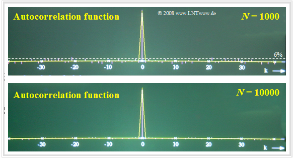
$\text{Beispiel 5:}$ Der entscheidende Parameter für die Qualität der numerischen AKF–Berechnung ist die Anzahl $N$ der berücksichtigten Abtastwerte.
- In der oberen Grafik sehen Sie das Ergebnis der numerischen AKF-Berechnung für $N = 1000$.
- Die untere Grafik gilt für $N = 10000$ Abtastwerte.
Die betrachteten Zufallsgrößen sind hier voneinander statistisch unabhängig. Somit sollten eigentlich alle AKF–Werte mit Ausnahme des Wertes bei $k = 0$ identisch Null sein.
- Bei $N = 10000$ (untere Grafik) beträgt der maximale Fehler nur noch etwa $1\%$ und ist bei dieser Darstellung fast nicht mehr sichtbar.
- Dagegen wächst der Fehler bei $N = 1000$ (obere Grafik) bis auf $±6\%$ an.
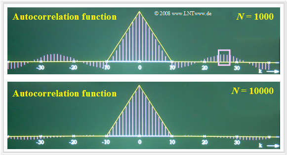
$\text{Beispiel 6:}$ Die Ergebnisse ändern sich, wenn eine Zufallsgröße mit inneren statistischen Bindungen vorliegt.
Betrachten wir beispielsweise eine dreieckförmige AKF mit $φ_x(k) ≠ 0$ für $\vert k \vert ≤ 10$, so erkennt man deutlich größere Abweichungen, nämlich
- Fehler bis zu etwa $±15\%$ bei $N = 1000$,
- Fehler bis zu etwa $±5\%$ bei $N = 10000$.
Begründung des schlechteren Ergebnisses gemäß $\text{Beispiel 6}$:
- Aufgrund der inneren statistischen Bindungen liefern nun nicht mehr alle Abtastwerte die volle Information über den zugrundeliegenden Zufallsprozess.
- Außerdem lassen die Bilder erkennen, dass bei der numerischen AKF–Berechnung einer Zufallsgröße mit statistischen Bindungen auch die Fehler korreliert sind.
- Ist – wie beispielsweise im oberen Bild zu sehen – der AKF-Wert $φ_x({\rm 26})$ fälschlicherweise positiv und groß, so ergeben sich auch die benachbarten AKF-Werte $φ_x({\rm 25})$ und $φ_x({\rm 27})$ als positiv und mit ähnlichen Zahlenwerten. Dieser Bereich ist in der oberen Grafik durch das Rechteck markiert.
Aufgaben zum Kapitel
Aufgabe 4.09Z: Periodische AKF
Aufgabe 4.10: Binär und quaternär
Aufgabe 4.10Z: Korrelationsdauer
Aufgabe 4.11: C-Programm „akf1”
Aufgabe 4.11Z: C-Programm „akf2”
