Difference between revisions of "Aufgaben:Exercise 4.10: Binary and Quaternary"
From LNTwww
| Line 1: | Line 1: | ||
| − | {{quiz-Header|Buchseite= | + | {{quiz-Header|Buchseite=Theory_of_Stochastic_Signals/Auto-Correlation_Function |
}} | }} | ||
| − | [[File:P_ID384__Sto_A_4_10.png|right|300px|frame| | + | [[File:P_ID384__Sto_A_4_10.png|right|300px|frame|Binary signal $b(t)$ and quaternary signal $q(t)$]] |
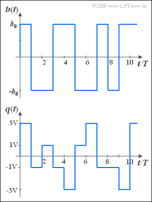
| − | + | We consider here a binärsignal $b(t)$ and a quaternaryärsignal $q(t)$, where: | |
| − | * | + | *The two signals are rectangular in shape, and the duration of each rectangle is $T$ (symbol duration). |
| − | * | + | *The symbols represented by the pulse heights of the individual rectangular pulses $($with step number $M = 2$ or $M = 4)$ are statistically independent. |
| − | * | + | *Because of the bipolar signal constellation, both signals are equal-signal-free if the symbol probabilities are chosen appropriately (symmetrically). |
| − | * | + | *Because of the latter property, it follows for the probabilities of the binary symbols: |
:$${\rm Pr}\big[b(t) = +b_0\big] = {\rm Pr}\big[b(t) = -b_0\big] ={1}/{2}.$$ | :$${\rm Pr}\big[b(t) = +b_0\big] = {\rm Pr}\big[b(t) = -b_0\big] ={1}/{2}.$$ | ||
| − | * | + | *In contrast, for the quarternärsignal: |
:$${\rm Pr}\big[q(t) = +3 \hspace{0.05cm}{\rm V}\big] = {\rm Pr}\big[q(t) = -3 \hspace{0.05cm}{\rm V}\big]= {1}/{6},$$ | :$${\rm Pr}\big[q(t) = +3 \hspace{0.05cm}{\rm V}\big] = {\rm Pr}\big[q(t) = -3 \hspace{0.05cm}{\rm V}\big]= {1}/{6},$$ | ||
:$${\rm Pr}\big[q(t) = +1 \hspace{0.05cm}{\rm V}\big] = {\rm Pr}\big[q(t) = -1 \hspace{0.05cm}{\rm V}\big]= {2}/{6}.$$ | :$${\rm Pr}\big[q(t) = +1 \hspace{0.05cm}{\rm V}\big] = {\rm Pr}\big[q(t) = -1 \hspace{0.05cm}{\rm V}\big]= {2}/{6}.$$ | ||
| Line 18: | Line 18: | ||
| − | + | Hint: | |
| − | * | + | *This exercise belongs to the chapter [[Theory_of_Stochastic_Signals/Auto-Correlation_Function|Auto-Correlation Function]]. |
| − | === | + | ===Questions=== |
<quiz display=simple> | <quiz display=simple> | ||
| − | { | + | {Calculate the AKF–value $\varphi_q(\tau = 0)$ of the quaternary signal. |
|type="{}"} | |type="{}"} | ||
| − | $\varphi_q(\tau = 0) \ = \ $ | + | $\varphi_q(\tau = 0) \ = \ $ { 3.667 3% } $\ \rm V^2$ |
| − | { | + | {What is the magnitude of the AKF–value when $\tau = T$ ? Justify why the AKF–values for $\tau| > T$ are the same size. Sketch the AKF–progression. |
|type="{}"} | |type="{}"} | ||
| − | $\varphi_q(\tau = T) \ = | + | $\varphi_q(\tau = T) \ = \ $ { 0. } $\ \rm V^2$ |
| − | { | + | {With which amplitude values $(\pm b_0)$ does the binary signal $b(t)$ have exactly the same ASF? |
|type="{}"} | |type="{}"} | ||
$b_0\ = \ $ { 1.915 3% } $\ \rm V$ | $b_0\ = \ $ { 1.915 3% } $\ \rm V$ | ||
| − | { | + | {Which of the following descriptive quantities of a stochastic process can be determined from the AKF? |
|type="[]"} | |type="[]"} | ||
| − | + | + | + period duration. |
| − | - | + | - Probability density function. |
| − | + | + | + Linear mean value. |
| − | + | + | + Variance. |
| − | - | + | - 3rd order moment. |
| − | - | + | -phase relations. |
| Line 56: | Line 56: | ||
</quiz> | </quiz> | ||
| − | === | + | ===Solution=== |
{{ML-Kopf}} | {{ML-Kopf}} | ||
| − | '''(1)''' | + | '''(1)''' The ACF value at the point $\tau = 0$ corresponds to the mean signal power, i.e. the root mean square value of $q(t)$. For this holds: |
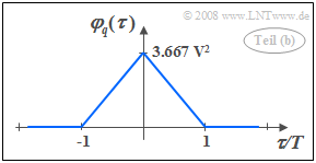
| − | [[File:P_ID385__Sto_A_4_10_b_neu.png|right|frame| | + | [[File:P_ID385__Sto_A_4_10_b_neu.png|right|frame|Triangular ACF]] |
| − | :$$\varphi_q(\tau = 0)= | + | :$$\varphi_q(\tau = 0)= {1}/{6 } \cdot ({\rm 3\,V})^2 + {2}/{6 } \cdot ({\rm 1\,V})^2 + {2}/{6 } \cdot (-{\rm 1\,V})^2 + {1}/{6 } \cdot (-{\rm 3\,V})^2= \rm {22}/{6 }\, \rm V^2\hspace{0.15cm}\underline{= \rm 3.667 \,V^2}.$$ |
| − | '''(2)''' | + | '''(2)''' The individual symbols were assumed to be statistically independent. |
| − | * | + | *Therefore, and because of the lack of a DC component, for any integer value of $\nu$, the following applies here: |
| − | :$${\rm E} \big [ q(t) \cdot q ( t + \nu T) \big ] = {\rm E} \big [ q(t) \big ] \cdot {\rm E} \big [ | + | :$${\rm E} \big [ q(t) \cdot q ( t + \nu T) \big ] = {\rm E} \big [ q(t) \big ] \cdot {\rm E} \big [ q ( t + \nu T) \big ]\hspace{0.15cm}\underline{ = 0}.$$ |
| − | * | + | *Thus, the ACF we are looking for has the shape sketched on the right. |
| − | * | + | *In the range $-T \le \tau \le +T$ the ACF is sectionwise linear, i.e. triangular, due to the rectangular pulse shape. |
<br clear=all> | <br clear=all> | ||
| − | '''(3)''' | + | '''(3)''' The ACF $\varphi_b(\tau)$ of the binary signal is also identically zero due to the statistically independent symbols in the range $| \tau| > T$ and for $-T \le \tau \le +T$ also results in a triangular shape. |
| − | * | + | *For the quadratic mean, one obtains: |
:$$\varphi_b (\tau = 0) = b_{\rm 0}^{\rm 2}.$$ | :$$\varphi_b (\tau = 0) = b_{\rm 0}^{\rm 2}.$$ | ||
| − | * | + | *With $b_0\hspace{0.15cm}\underline{= 1.915\, \rm V}$ the two autocorrelation functions $\varphi_q(\tau)$ and $\varphi_b(\tau)$ are identical. |
| − | '''(4)''' | + | '''(4)''' Correct are <u>the proposed solutions 1, 3, and 4</u>. |
| − | + | From the autocorrelation function we can actually determine: | |
| − | * | + | *the period $T_0$: this is the same for the pattern signals and the ACF; |
| − | * | + | * the linear mean: root of the final value of the ACF for $\tau \to \infty$ and |
| − | * | + | * the variance: difference of the ACF values of $\tau = 0$ and $\tau \to \infty$. |
| − | + | Cannot be determined: | |
| − | * | + | * the probability density function: despite $\varphi_q(\tau) =\varphi_b(\tau)$ is $f_q(q) \ne f_b(b)$; |
| − | * | + | * the moments of higher order: for their calculation one needs the PDF; |
| − | * | + | * All phase relations and symmetry properties are not recognizable from the ACF. |
{{ML-Fuß}} | {{ML-Fuß}} | ||
Revision as of 22:49, 28 February 2022
We consider here a binärsignal $b(t)$ and a quaternaryärsignal $q(t)$, where:
- The two signals are rectangular in shape, and the duration of each rectangle is $T$ (symbol duration).
- The symbols represented by the pulse heights of the individual rectangular pulses $($with step number $M = 2$ or $M = 4)$ are statistically independent.
- Because of the bipolar signal constellation, both signals are equal-signal-free if the symbol probabilities are chosen appropriately (symmetrically).
- Because of the latter property, it follows for the probabilities of the binary symbols:
- $${\rm Pr}\big[b(t) = +b_0\big] = {\rm Pr}\big[b(t) = -b_0\big] ={1}/{2}.$$
- In contrast, for the quarternärsignal:
- $${\rm Pr}\big[q(t) = +3 \hspace{0.05cm}{\rm V}\big] = {\rm Pr}\big[q(t) = -3 \hspace{0.05cm}{\rm V}\big]= {1}/{6},$$
- $${\rm Pr}\big[q(t) = +1 \hspace{0.05cm}{\rm V}\big] = {\rm Pr}\big[q(t) = -1 \hspace{0.05cm}{\rm V}\big]= {2}/{6}.$$
Hint:
- This exercise belongs to the chapter Auto-Correlation Function.
Questions
Solution
(1) The ACF value at the point $\tau = 0$ corresponds to the mean signal power, i.e. the root mean square value of $q(t)$. For this holds:
- $$\varphi_q(\tau = 0)= {1}/{6 } \cdot ({\rm 3\,V})^2 + {2}/{6 } \cdot ({\rm 1\,V})^2 + {2}/{6 } \cdot (-{\rm 1\,V})^2 + {1}/{6 } \cdot (-{\rm 3\,V})^2= \rm {22}/{6 }\, \rm V^2\hspace{0.15cm}\underline{= \rm 3.667 \,V^2}.$$
(2) The individual symbols were assumed to be statistically independent.
- Therefore, and because of the lack of a DC component, for any integer value of $\nu$, the following applies here:
- $${\rm E} \big [ q(t) \cdot q ( t + \nu T) \big ] = {\rm E} \big [ q(t) \big ] \cdot {\rm E} \big [ q ( t + \nu T) \big ]\hspace{0.15cm}\underline{ = 0}.$$
- Thus, the ACF we are looking for has the shape sketched on the right.
- In the range $-T \le \tau \le +T$ the ACF is sectionwise linear, i.e. triangular, due to the rectangular pulse shape.
(3) The ACF $\varphi_b(\tau)$ of the binary signal is also identically zero due to the statistically independent symbols in the range $| \tau| > T$ and for $-T \le \tau \le +T$ also results in a triangular shape.
- For the quadratic mean, one obtains:
- $$\varphi_b (\tau = 0) = b_{\rm 0}^{\rm 2}.$$
- With $b_0\hspace{0.15cm}\underline{= 1.915\, \rm V}$ the two autocorrelation functions $\varphi_q(\tau)$ and $\varphi_b(\tau)$ are identical.
(4) Correct are the proposed solutions 1, 3, and 4.
From the autocorrelation function we can actually determine:
- the period $T_0$: this is the same for the pattern signals and the ACF;
- the linear mean: root of the final value of the ACF for $\tau \to \infty$ and
- the variance: difference of the ACF values of $\tau = 0$ and $\tau \to \infty$.
Cannot be determined:
- the probability density function: despite $\varphi_q(\tau) =\varphi_b(\tau)$ is $f_q(q) \ne f_b(b)$;
- the moments of higher order: for their calculation one needs the PDF;
- All phase relations and symmetry properties are not recognizable from the ACF.

