Difference between revisions of "Aufgaben:Exercise 4.12Z: White Gaussian Noise"
| (2 intermediate revisions by the same user not shown) | |||
| Line 11: | Line 11: | ||
The bottom graph shows the two power-spectral densities ${\it \Phi}_{b}(f)$ and ${\it \Phi}_{b+}(f)$ of bandlimited white noise signal $b(t)$. It holds with the one-sided bandwidth $B$: | The bottom graph shows the two power-spectral densities ${\it \Phi}_{b}(f)$ and ${\it \Phi}_{b+}(f)$ of bandlimited white noise signal $b(t)$. It holds with the one-sided bandwidth $B$: | ||
| − | :$${\it \Phi}_b(f)=\left\{ {N_0/2\atop 0}{\hspace{0.5cm} {\rm | + | :$${\it \Phi}_b(f)=\left\{ {N_0/2\atop 0}{\hspace{0.5cm} {\rm for}\quad |f|\le B \atop {\rm else}}\right.,$$ |
| − | :$${\it \Phi}_{b+}(f)=\left\{ {N_0\atop 0}{\hspace{0.5cm} {\rm | + | :$${\it \Phi}_{b+}(f)=\left\{ {N_0\atop 0}{\hspace{0.5cm} {\rm for}\quad 0 \le f\le B \atop {\rm else}}\right.$$ |
For computer simulation of noise processes, band-limited noise must always be assumed, since only discrete-time processes can be handled. For this, the [[Signal_Representation/Discrete-Time_Signal_Representation#Sampling_theorem|Sampling Theorem]] must be obeyed. This states that the bandwidth $B$ must be set according to the interpolation distance $T_{\rm A}$ of the simulation. | For computer simulation of noise processes, band-limited noise must always be assumed, since only discrete-time processes can be handled. For this, the [[Signal_Representation/Discrete-Time_Signal_Representation#Sampling_theorem|Sampling Theorem]] must be obeyed. This states that the bandwidth $B$ must be set according to the interpolation distance $T_{\rm A}$ of the simulation. | ||
| Line 29: | Line 29: | ||
Hints: | Hints: | ||
*This exercise belongs to the chapter [[Theory_of_Stochastic_Signals/Power-Spectral_Density|Power-Spectral Density]]. | *This exercise belongs to the chapter [[Theory_of_Stochastic_Signals/Power-Spectral_Density|Power-Spectral Density]]. | ||
| − | *Reference is also made to the chapter [[Theory_of_Stochastic_Signals/Auto-Correlation_Function|Auto- | + | *Reference is also made to the chapter [[Theory_of_Stochastic_Signals/Auto-Correlation_Function|Auto-Correlation Function]]. |
*The properties of white noise are summarized in the second part of the (German language) learning video [[Der_AWGN-Kanal_(Lernvideo)|The AWGN channel]]. | *The properties of white noise are summarized in the second part of the (German language) learning video [[Der_AWGN-Kanal_(Lernvideo)|The AWGN channel]]. | ||
| Line 74: | Line 74: | ||
===Solution=== | ===Solution=== | ||
{{ML-Kopf}} | {{ML-Kopf}} | ||
| − | '''(1)''' Correct are <u>solutions 2, 3, and 4</u>: | + | '''(1)''' Correct are the <u>solutions 2, 3, and 4</u>: |
| − | *The auto-correlation function (ACF) is the Fourier transform of the | + | *The auto-correlation function $\rm (ACF)$ is the Fourier transform of the power-spectral density $\rm (PSD)$. Here: |
:$${\it \Phi}_n (f) = {N_0}/{2} \hspace{0.3cm} \bullet\!\!-\!\!\!-\!\!\!-\!\!\circ\, \hspace{0.3cm} \varphi_n (\tau)={N_0}/{2} \cdot {\rm \delta} ( \tau).$$ | :$${\it \Phi}_n (f) = {N_0}/{2} \hspace{0.3cm} \bullet\!\!-\!\!\!-\!\!\!-\!\!\circ\, \hspace{0.3cm} \varphi_n (\tau)={N_0}/{2} \cdot {\rm \delta} ( \tau).$$ | ||
| − | *However, there is no "real" white noise in physics, since such a noise would have to have an infinitely large signal power $($the integral over the PSD as well as the ACF value at $\tau = 0$ are both infinitely large$)$. | + | *However, there is no "real" white noise in physics, since such a noise would have to have an infinitely large signal power $($the integral over the PSD as well as the ACF value at $\tau = 0$ are both infinitely large$)$. |
| − | *Thermal noise has a constant PSD up to frequencies of about $\text{6000 GHz}$ | + | *Thermal noise has a constant PSD up to frequencies of about $\text{6000 GHz}$. Since all (current) transmission systems operate in a much lower frequency range, thermal noise can be said to be "white" to a good approximation. |
| − | *The statistical property "white" says nothing about the amplitude distribution, which is determined by the probability density function (PDF) alone. | + | *The statistical property "white" says nothing about the amplitude distribution, which is determined by the probability density function $\rm (PDF)$ alone. |
| − | *When considering the phase of a bandpass signal as the stochastic variable, it is often modeled as uniformly distributed between $0$ and $2\pi$ | + | *When considering the phase of a bandpass signal as the stochastic variable, it is often modeled as uniformly distributed between $0$ and $2\pi$. |
| − | *If there are no statistical bindings between the respective phase angles at different times, this random process is also "white". | + | *If there are no statistical bindings between the respective phase angles at different times, this random process is also "white". |
| − | |||
| − | |||
| − | |||
| − | |||
[[File:P_ID410__Sto_Z_4_12_b.png|right|frame|ACF of band-limited noise]] | [[File:P_ID410__Sto_Z_4_12_b.png|right|frame|ACF of band-limited noise]] | ||
| − | '''(2)''' The | + | '''(2)''' The power-spectral density is a rectangle of width $2B$ and height $N_0/2$. |
| − | *The inverse Fourier | + | *The inverse Fourier transform yields an sinc–function: |
:$$\varphi_b(\tau) = N_0 \cdot B \cdot {\rm si} (2 \pi B \tau)\hspace{0.3cm} | :$$\varphi_b(\tau) = N_0 \cdot B \cdot {\rm si} (2 \pi B \tau)\hspace{0.3cm} | ||
\Rightarrow \hspace{0.3cm}\varphi_b(\tau = 0) = N_0 \cdot B \hspace{0.15cm}\underline {=4}\cdot 10^{-6} \ \rm V^2.$$ | \Rightarrow \hspace{0.3cm}\varphi_b(\tau = 0) = N_0 \cdot B \hspace{0.15cm}\underline {=4}\cdot 10^{-6} \ \rm V^2.$$ | ||
| Line 97: | Line 93: | ||
'''(3)''' The ACF value at the point $\tau = 0$ gives the power. | '''(3)''' The ACF value at the point $\tau = 0$ gives the power. | ||
| − | *The root of this is called the rms value: | + | *The root of this is called the "rms value": |
:$$\sigma_b = \sqrt{\varphi_b(\tau = 0)} \hspace{0.15cm}\underline {=2 \hspace{0.05cm}\rm V}.$$ | :$$\sigma_b = \sqrt{\varphi_b(\tau = 0)} \hspace{0.15cm}\underline {=2 \hspace{0.05cm}\rm V}.$$ | ||
| + | |||
| + | |||
'''(4)''' The ACF computed in '''(3)''' has zeros at equidistant distance from $T_{\rm A}= 1/(2B)\hspace{0.15cm}\underline {=5\hspace{0.05cm} \rm ns}$: | '''(4)''' The ACF computed in '''(3)''' has zeros at equidistant distance from $T_{\rm A}= 1/(2B)\hspace{0.15cm}\underline {=5\hspace{0.05cm} \rm ns}$: | ||
*There are no statistical bindings between the two signal values $b(t)$ and $b(t + \nu \cdot T_{\rm A})$, | *There are no statistical bindings between the two signal values $b(t)$ and $b(t + \nu \cdot T_{\rm A})$, | ||
| Line 105: | Line 103: | ||
| − | '''(5)''' The correct solution is <u>suggested solution 2</u>. | + | '''(5)''' The correct solution is the <u>suggested solution 2</u>. |
| − | *The ACF value at $\tau = T_{\rm A} = 1 \hspace{0.05cm}\rm ns$ | + | *The ACF value at $\tau = T_{\rm A} = 1 \hspace{0.05cm}\rm ns$ is |
| − | :$$\varphi_b(\tau = T_{\rm A}) = {\rm 4 \cdot 10^{-6} \hspace{0.1cm}V^2 \cdot | + | :$$\varphi_b(\tau = T_{\rm A}) = {\rm 4 \cdot 10^{-6} \hspace{0.1cm}V^2 \cdot sinc (1/5) \approx 3.742 \cdot 10^{-6} \hspace{0.1cm}V^2} > 0.$$ |
*This result says: Two signal values separated by $T_{\rm A} = 1 \hspace{0.05cm}\rm ns$ are positively correlated: | *This result says: Two signal values separated by $T_{\rm A} = 1 \hspace{0.05cm}\rm ns$ are positively correlated: | ||
| − | *If $b(t)$ is positive and large; | + | :*If $b(t)$ is positive and large, then with high probability $b(t+1 \hspace{0.05cm}\rm ns)$ is also positive and large. |
| − | *In contrast, there is a negative correlation between $b(t)$ and $b(t+7 \hspace{0.05cm}\rm ns)$ If $b(t)$ is positive, then $b(t+7 \hspace{0.05cm}\rm ns)$ is probably negative. | + | :*In contrast, there is a negative correlation between $b(t)$ and $b(t+7 \hspace{0.05cm}\rm ns)$. If $b(t)$ is positive, then $b(t+7 \hspace{0.05cm}\rm ns)$ is probably negative. |
{{ML-Fuß}} | {{ML-Fuß}} | ||
Latest revision as of 15:27, 25 March 2022
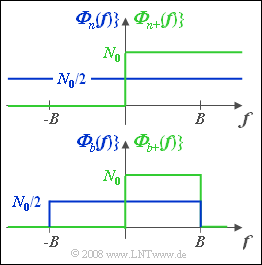
A noise signal $n(t)$ is called "white" if it contains all spectral components without preference of any frequencies.
- The physical power-spectral density defined only for positive frequencies ⇒ ${\it \Phi}_{n+}(f)$ is constant $($equal $N_0)$ and extends frequency-wise to infinity.
- ${\it \Phi}_{n+}(f)$ is shown in green in the upper graph. The plus sign in the index is to indicate that the function is valid only for positive values of $f$.
- For mathematical description one usually uses the two-sided power-spectral density ${\it \Phi}_{n}(f)$. Here applies for all frequencies from $-\infty$ to $+\infty$ (blue curve in the upper graph):
- $${\it \Phi}_n (f) ={N_0}/{2}.$$
The bottom graph shows the two power-spectral densities ${\it \Phi}_{b}(f)$ and ${\it \Phi}_{b+}(f)$ of bandlimited white noise signal $b(t)$. It holds with the one-sided bandwidth $B$:
- $${\it \Phi}_b(f)=\left\{ {N_0/2\atop 0}{\hspace{0.5cm} {\rm for}\quad |f|\le B \atop {\rm else}}\right.,$$
- $${\it \Phi}_{b+}(f)=\left\{ {N_0\atop 0}{\hspace{0.5cm} {\rm for}\quad 0 \le f\le B \atop {\rm else}}\right.$$
For computer simulation of noise processes, band-limited noise must always be assumed, since only discrete-time processes can be handled. For this, the Sampling Theorem must be obeyed. This states that the bandwidth $B$ must be set according to the interpolation distance $T_{\rm A}$ of the simulation.
Assume the following numerical values throughout this exercise:
- The noise power density – with respect to the resistor $1 \hspace{0.05cm}\rm \Omega$ – is $N_0 = 4 \cdot 10^{-14}\hspace{0.05cm}\rm V^2/Hz$.
- The (one-sided) bandwidth of the band-limited white noise is $B = 100 \hspace{0.08cm}\rm MHz$.
Hints:
- This exercise belongs to the chapter Power-Spectral Density.
- Reference is also made to the chapter Auto-Correlation Function.
- The properties of white noise are summarized in the second part of the (German language) learning video The AWGN channel.
Questions
Solution
- The auto-correlation function $\rm (ACF)$ is the Fourier transform of the power-spectral density $\rm (PSD)$. Here:
- $${\it \Phi}_n (f) = {N_0}/{2} \hspace{0.3cm} \bullet\!\!-\!\!\!-\!\!\!-\!\!\circ\, \hspace{0.3cm} \varphi_n (\tau)={N_0}/{2} \cdot {\rm \delta} ( \tau).$$
- However, there is no "real" white noise in physics, since such a noise would have to have an infinitely large signal power $($the integral over the PSD as well as the ACF value at $\tau = 0$ are both infinitely large$)$.
- Thermal noise has a constant PSD up to frequencies of about $\text{6000 GHz}$. Since all (current) transmission systems operate in a much lower frequency range, thermal noise can be said to be "white" to a good approximation.
- The statistical property "white" says nothing about the amplitude distribution, which is determined by the probability density function $\rm (PDF)$ alone.
- When considering the phase of a bandpass signal as the stochastic variable, it is often modeled as uniformly distributed between $0$ and $2\pi$.
- If there are no statistical bindings between the respective phase angles at different times, this random process is also "white".
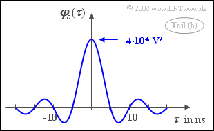
(2) The power-spectral density is a rectangle of width $2B$ and height $N_0/2$.
- The inverse Fourier transform yields an sinc–function:
- $$\varphi_b(\tau) = N_0 \cdot B \cdot {\rm si} (2 \pi B \tau)\hspace{0.3cm} \Rightarrow \hspace{0.3cm}\varphi_b(\tau = 0) = N_0 \cdot B \hspace{0.15cm}\underline {=4}\cdot 10^{-6} \ \rm V^2.$$
(3) The ACF value at the point $\tau = 0$ gives the power.
- The root of this is called the "rms value":
- $$\sigma_b = \sqrt{\varphi_b(\tau = 0)} \hspace{0.15cm}\underline {=2 \hspace{0.05cm}\rm V}.$$
(4) The ACF computed in (3) has zeros at equidistant distance from $T_{\rm A}= 1/(2B)\hspace{0.15cm}\underline {=5\hspace{0.05cm} \rm ns}$:
- There are no statistical bindings between the two signal values $b(t)$ and $b(t + \nu \cdot T_{\rm A})$,
- where $\nu$ can take all integer values.
(5) The correct solution is the suggested solution 2.
- The ACF value at $\tau = T_{\rm A} = 1 \hspace{0.05cm}\rm ns$ is
- $$\varphi_b(\tau = T_{\rm A}) = {\rm 4 \cdot 10^{-6} \hspace{0.1cm}V^2 \cdot sinc (1/5) \approx 3.742 \cdot 10^{-6} \hspace{0.1cm}V^2} > 0.$$
- This result says: Two signal values separated by $T_{\rm A} = 1 \hspace{0.05cm}\rm ns$ are positively correlated:
- If $b(t)$ is positive and large, then with high probability $b(t+1 \hspace{0.05cm}\rm ns)$ is also positive and large.
- In contrast, there is a negative correlation between $b(t)$ and $b(t+7 \hspace{0.05cm}\rm ns)$. If $b(t)$ is positive, then $b(t+7 \hspace{0.05cm}\rm ns)$ is probably negative.

