Aufgaben:Exercise 4.4: About the Quantization Noise

• Return to book

Quantization error with sawtooth input

To calculate the quantization noise power  $P_{\rm Q}$  we assume a periodic sawtooth-shaped source signal  $q(t)$  with value range  $±q_{\rm max}$  and period duration  $T_0$ .

• In the mean time domain  $-T_0/2 ≤ t ≤ T_0/2$  holds:   $q(t) = q_{\rm max} \cdot \left ( {2 \cdot t}/{T_0} \right ).$
• We refer to the power of the signal  $q(t)$  here as the transmit power  $P_{\rm S}$.

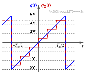
The signal  $q(t)$  is quantized according to the graph with  $M = 6$  steps.  The quantized signal is  $q_{\rm Q}(t)$,  where:

• The linear quantizer is designed for the amplitude range  $±Q_{\rm max}$  such that each quantization interval has width  ${\it Δ} = 2/M \cdot Q_{\rm max}$.
• The diagram shows this fact for  $Q_{\rm max} = q_{\rm max} = 6 \ \rm V$.  These numerical values shall be assumed up to and including the subtask  (5).

The  "quantization noise power"  is defined as the second moment of the difference signal  $ε(t) = q_{\rm Q}(t) - q(t)$.  It holds:

$$P_{\rm Q} = \frac{1}{T_0' } \cdot \int_{0}^{T_0'}\varepsilon(t)^2 \hspace{0.05cm}{\rm d}t \hspace{0.05cm},$$

where the time  $T_0'$  is to be chosen appropriately.  The  "quantization SNR"  is the ratio    $\rho_{\rm Q} = {P_{\rm S}}/{P_{\rm Q}}\hspace{0.05cm}$,  which is usually given logarithmically  (in dB).

Hints:

• The exercise belongs to the chapter  "Pulse Code Modulation".
• Reference is made in particular to the page  "Quantization and quantization Noise".

Questions

1

Calculate the signal power  $P_{\rm S}$  $($referred to the resistor $1 \ \rm Ω)$.

$P_{\rm S} \ = \ $ $\ \rm V^2$

2

Which statements are true for the error signal  $ε(t)$ ?

	$ε(t)$  has a sawtooth shape.
	$ε(t)$  has a step-like progression.
	$ε(t)$  is restricted to the range  $±{\it Δ}/2 = ±1 \ \rm V$.
	$ε(t)$  has period  $T_0' = T_0/M$.

3

What is the quantization noise power  $P_{\rm Q}$  for  $M=6$?

$P_{\rm Q} \ = \ $ $\ \rm V^2$

4

Calculate the quantization noise ratio for  $M = 6$.

$10 \cdot \lg \ ρ_{\rm Q} \ = \ $ $\ \rm dB$

5

What values result from quantization with  $N = 8$  or  $N = 16$ bits?

$N = 8\text{:}\hspace{0.35cm}10 ⋅ \lg \ ρ_{\rm Q} \ = \ $ $\ \rm dB$

$N = 16\text{:}\hspace{0.15cm}10 ⋅ \lg \ ρ_{\rm Q} \ = \ $ $\ \rm dB$

6

What conditions must be met for the derived equation to apply to  $ρ_{\rm Q}$?

	All amplitude values are equally probable.
	A linear quantizer is present.
	The quantizer is exactly matched to the signal  $(Q_{\rm max} = q_{\rm max})$.

Solution

Solution

(1)  The signal power  $P_{\rm S} $  is equal to the root mean square of  $q(t)$ if the reference resistance  $1 \rm Ω$  is used and therefore the unit  $\rm V^2$  is accepted for the power.

• Due to periodicity and symmetry, averaging over the time domain  $T_0/2$ is sufficient:

$$P_{\rm S} = \frac{1}{T_0/2} \cdot \int_{0}^{T_0/2}q^2(t) \hspace{0.05cm}{\rm d}t = \frac{2 \cdot q_{\rm max}^2}{T_0} \cdot \int_{0}^{T_0/2}\left ( { 2 \cdot t}/{T_0} \right )^2 \hspace{0.05cm}{\rm d}t= \frac{2 \cdot q_{\rm max}^2}{T_0} \cdot \frac{T_0}{2} \cdot \int_{0}^{1}x^2 \hspace{0.05cm}{\rm d}x = \frac{q_{\rm max}^2}{3} \hspace{0.05cm}.$$

• Here the substitution  $x = 2 - t/T_0$  was used.  With  $q_{\rm max} = 6 \ \rm V$  one gets  $P_\rm S\hspace{0.15cm}\underline { = 12 \ V^2}$.

Error signal for  $Q_{\rm max} = q_{\rm max}$

(2)  Correct are suggested solutions 1, 3, and 4:

• We assume here  $Q_{\rm max} = q_{\rm max} = 6 \ \rm V$  .
• This gives the sawtooth-shaped error signal  $ε(t)$  between  $±1\ \rm V$.
• The period duration is  $T_0' = T_0/6$.

(3)  The error signal  $ε(t)$  proceeds in the same way as  $q(t)$  sawtooth.

• Thus, the same equation as in subtask  (1)' is suitable for calculating the root mean square.
• Note, however, that the amplitude is smaller by a factor  $M$  while the different period duration does not matter for the averaging:

$$P_{\rm Q} = \frac{P_{\rm S}}{M^2} = \frac{12\,{\rm V}^2}{36}\hspace{0.15cm}\underline {= 0.333\,{\rm V}^2 }\hspace{0.05cm}.$$

(4)  The results of the subtasks  (1)  and  (3)  lead to the quantization SNR:

$$\rho_{\rm Q} = \frac{P_{\rm S}}{P_{\rm Q}} = M^2 = 36 \hspace{0.3cm}\Rightarrow \hspace{0.3cm} 10 \cdot {\rm lg}\hspace{0.1cm}\rho_{\rm Q}\hspace{0.15cm}\underline { =15.56\,{\rm dB}} \hspace{0.05cm}.$$

(5)  With  $M = 2^N$  we obtain in general:

$$ \rho_{\rm Q} = M^2 = 2^{2N} \hspace{0.3cm}\rightarrow \hspace{0.3cm} 10 \cdot {\rm lg}\hspace{0.1cm}\rho_{\rm Q} =20 \cdot {\rm lg}\hspace{0.1cm}(2)\cdot N \approx 6.02\,{\rm dB} \cdot N .$$

• This results in the special cases we are looking for:

$$N = 8:\hspace{0.2cm} 10 \cdot {\rm lg}\hspace{0.1cm}\rho_{\rm Q} \hspace{0.15cm}\underline {= 48.16\,{\rm dB}}\hspace{0.05cm},$$

$$N = 16:\hspace{0.2cm} 10 \cdot {\rm lg}\hspace{0.1cm}\rho_{\rm Q} \hspace{0.15cm}\underline { = 96.32\,{\rm dB}}\hspace{0.05cm}.$$

(6)  All of the above preconditions must be satisfied:

• For nonlinear quantization, the simple relation  $ρ_{\rm Q} = M^2$  does not hold.
• For an amplitude distribution other than the uniform distribution  $ρ_{\rm Q} = M^2$  is also only an approximation, but this is usually accepted.
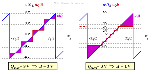
• If  $Q_{\rm max} < q_{\rm max}$, truncation of the peaks occurs, while with  $Q_{\rm max} > q_{\rm max}$  the quantization intervals are larger than required.

Quantization with  $Q_{\rm max} \ne q_{\rm max}$

The graph shows the error signals  $ε(t)$  for  $Q_{\rm max} > q_{\rm max}$  (left) and  $Q_{\rm max} < q_{\rm max}$  (right).

In both cases, the quantization noise power is significantly larger than calculated in point  (3) .