Difference between revisions of "Aufgaben:Exercise 4.5: Non-Linear Quantization"
m (Guenter verschob die Seite 4.5 Nichtlineare Quantisierung nach Aufgabe 4.5: Nichtlineare Quantisierung) |
|||
| (14 intermediate revisions by 4 users not shown) | |||
| Line 1: | Line 1: | ||
| − | {{quiz-Header|Buchseite= | + | {{quiz-Header|Buchseite=Modulation_Methods/Pulse_Code_Modulation |
}} | }} | ||
| − | [[File: | + | [[File:EN_Mod_Z_4_5.png|right|frame|PCM system with companding]] |
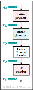
| − | + | To investigate "non-linear quantization" we start from the outlined system model. | |
| + | *We disregard the influence of the channel and the PCM coding or decoding. | ||
| + | *Thus, $v_{\rm Q}(ν \cdot T_{\rm A}) = q_{\rm Q}(ν \cdot T_{\rm A})$ always applies, whereby the time specification $ν \cdot T_{\rm A}$ is omitted in the following. | ||
| − | |||
| − | |||
| − | |||
| − | |||
| − | |||
| − | |||
| + | By comparing one output variable with one input variable at the same time, it is possible to determine the influence | ||
| + | * of the compressor ⇒ $q_{\rm K}(q_{\rm A})$, | ||
| + | * of the linear quantizer ⇒ $q_{\rm Q}(q_{\rm K})$, | ||
| + | * of the non-linear quantizer ⇒ $q_{\rm Q}(q_{\rm A})$, | ||
| + | * of the expander ⇒ $v_{\rm E}(v_{\rm Q})$, and | ||
| + | * of the overall system ⇒ $v_{\rm E}(q_{\rm A})$. | ||
| − | |||
| − | + | The following assumptions are made: | |
| − | |||
| − | |||
| + | * All samples $q_{\rm A}$ are in the value range $±1$ . | ||
| + | * The (linear) quantizer works with $M = 256$ quantization levels, which are marked with $μ = 0$ to $μ = 255$ . | ||
| + | * For compression, the so-called "13-segment" characteristic is used. | ||
| − | |||
| − | |||
| − | |||
| − | |||
| − | |||
| + | This means: | ||
| + | *In the range $|q_{\rm A}| ≤ 1/64$ holds $q_{\rm K} = q_{\rm A}$. | ||
| + | *For $q_{\rm A} > 1/64$, there are the following six additional ranges $(k = 1$, ... , $6)$ of the compressor characteristic: <br> ⇒ range $k\hspace{0.3cm}{\rm (if}\hspace{0.3cm} 2^{k-7}< q_{\rm A} \le 2^{k-6}) \hspace{0.05cm}$ ⇒ $q_{\rm K}(q_{\rm A}) = 2^{4-k} \cdot q_{\rm A} + {k}/{8}.$ | ||
| + | *Another six domains exist for negative $q_{\rm A}$ values with $k = -1$, ... , $-6$, which are point-symmetric with respect to the origin. <br>However, these are not considered further in this exercise. | ||
| − | |||
| − | |||
| − | |||
| − | |||
| − | === | + | |
| + | |||
| + | Hints: | ||
| + | *The exercise belongs to the chapter [[Modulation_Methods/Pulse_Code_Modulation|"Pulse Code Modulation]]. | ||
| + | *Reference is made in particular to the section [[Modulation_Methods/Pulse_Code_Modulation#Compression_and_expansion|"Compression and Expansion"]]. | ||
| + | |||
| + | |||
| + | |||
| + | ===Questions=== | ||
<quiz display=simple> | <quiz display=simple> | ||
| − | { | + | {If $q_{\rm A} = 0.4$: What is the output value $q_{\rm K}$ of the compressor? |
|type="{}"} | |type="{}"} | ||
$q_{\rm K} \ = \ $ { 0.825 3% } | $q_{\rm K} \ = \ $ { 0.825 3% } | ||
| − | { | + | { To which quantization interval $μ$ does $q_{\rm A} = 0.4$ belong? |
|type="{}"} | |type="{}"} | ||
$\mu \ = \ $ { 233 } | $\mu \ = \ $ { 233 } | ||
| − | { | + | {Which quantization value $q_{\rm Q}$ belongs to $q_{\rm A} = 0.4$? |
|type="{}"} | |type="{}"} | ||
$q_{\rm Q} \ = \ $ { 0.824 3% } | $q_{\rm Q} \ = \ $ { 0.824 3% } | ||
| − | { | + | {In contrast, what quantization value $q_{\rm Q}$ belongs to $q_{\rm A} = 0.04$? |
|type="{}"} | |type="{}"} | ||
$q_{\rm Q} \ = \ $ { 0.41 3% } | $q_{\rm Q} \ = \ $ { 0.41 3% } | ||
| − | { | + | {At the receiver, the input value is $v_{\rm Q} = 211/256 ≈ 0.824$. What value $v_{\rm E}$ does the expander provide? |
|type="{}"} | |type="{}"} | ||
$v_{\rm E} \ = \ $ { 0.398 3% } | $v_{\rm E} \ = \ $ { 0.398 3% } | ||
| − | { | + | {What are the properties of the "non-linear quantizer characteristic" $q_{\rm Q}(q_{\rm A})$ ? |
|type="[]"} | |type="[]"} | ||
| − | + | + | + The characteristic $q_{\rm Q}(q_{\rm A})$ approximates the compressor characteristic in steps. |
| − | - | + | - The characteristic $q_{\rm Q}(q_{\rm A})$ approximates the angle bisector in steps. |
| − | - | + | - The step width is the same in all segments $($except for $k = 0)$ . |
| − | + | + | + The step height is equal in all segments $($except for $k = 0)$ . |
| − | { | + | {What are the properties of the "overall system characteristic" $v_{\rm E}(q_{\rm A})$ ? |
|type="[]"} | |type="[]"} | ||
| − | - | + | - The characteristic $v_{\rm E}(q_{\rm A})$ approximates the compressor characteristic in steps. |
| − | + | + | + The characteristic $v_{\rm E}(q_{\rm A})$ approximates the angle bisector in steps. |
| − | - | + | - The step width is the same in all segments $($except for $k = 0)$ . |
| − | - | + | - The step height is equal in all segments $($except for $k = 0)$ . |
</quiz> | </quiz> | ||
| − | === | + | ===Solution=== |
{{ML-Kopf}} | {{ML-Kopf}} | ||
| − | '''(1)''' | + | '''(1)''' The sample $q_{\rm A} = 0.4$ belongs to the segment $k = 5$ covering the range $1/4 < q_{\rm A} ≤ 1/2$. From the given equation it follows that with $k = 5$: |
:$$q_{\rm K}(q_{\rm A}) = 2^{4-k} \cdot q_{\rm A} + {k}/{8}={1}/{2}\cdot 0.4 + {5}/{8} \hspace{0.15cm}\underline {= 0.825}\hspace{0.05cm}.$$ | :$$q_{\rm K}(q_{\rm A}) = 2^{4-k} \cdot q_{\rm A} + {k}/{8}={1}/{2}\cdot 0.4 + {5}/{8} \hspace{0.15cm}\underline {= 0.825}\hspace{0.05cm}.$$ | ||
| − | '''(2)''' | + | |
| + | |||
| + | '''(2)''' The input value of the linear quantizer is now $q_{\rm K} = 0.825$, so the following calculation applies: | ||
:$${105}/{128} < q_{\rm K} = 0.825 \le {106}/{128}\hspace{0.3cm}\Rightarrow \hspace{0.3cm} m = 105 \hspace{0.3cm}\Rightarrow \hspace{0.3cm} \mu = 128 + 105\hspace{0.15cm}\underline { = 233} \hspace{0.05cm}.$$ | :$${105}/{128} < q_{\rm K} = 0.825 \le {106}/{128}\hspace{0.3cm}\Rightarrow \hspace{0.3cm} m = 105 \hspace{0.3cm}\Rightarrow \hspace{0.3cm} \mu = 128 + 105\hspace{0.15cm}\underline { = 233} \hspace{0.05cm}.$$ | ||
| − | '''(3)''' | + | |
| − | $q_{\rm Q} = 1/256 + m/128$ | + | |
| + | '''(3)''' According to the specification page, the quantization interval $μ = 128 + m$ is given by the value | ||
| + | $q_{\rm Q} = 1/256 + m/128$. With $m = 105$ it follows: | ||
:$$q_{\rm Q} = \frac{1}{256} + \frac{105}{128} \hspace{0.15cm}\underline {\approx 0.824} \hspace{0.05cm}.$$ | :$$q_{\rm Q} = \frac{1}{256} + \frac{105}{128} \hspace{0.15cm}\underline {\approx 0.824} \hspace{0.05cm}.$$ | ||
| − | '''(4)''' | + | |
| + | |||
| + | '''(4)''' According to the sample solution to subtask '''(3)''' with the input value $q_{\rm A} = 0.04$: | ||
:$$ \frac{1}{32} < q_{\rm A} \le \frac{1}{16}\hspace{0.3cm}\Rightarrow \hspace{0.3cm} k = 2 \hspace{0.3cm}\Rightarrow \hspace{0.3cm} q_{\rm K} = 2^2 \cdot 0.04 + \frac{2}{8}= 0.41$$ | :$$ \frac{1}{32} < q_{\rm A} \le \frac{1}{16}\hspace{0.3cm}\Rightarrow \hspace{0.3cm} k = 2 \hspace{0.3cm}\Rightarrow \hspace{0.3cm} q_{\rm K} = 2^2 \cdot 0.04 + \frac{2}{8}= 0.41$$ | ||
:$$\Rightarrow \hspace{0.3cm}\frac{52}{128} < q_{\rm K} = 0.41 \le \frac{53}{128}\hspace{0.3cm}\Rightarrow \hspace{0.3cm} m = 52 \hspace{0.3cm}\Rightarrow \hspace{0.3cm} \mu = 128 + 52 = 180\hspace{0.3cm} | :$$\Rightarrow \hspace{0.3cm}\frac{52}{128} < q_{\rm K} = 0.41 \le \frac{53}{128}\hspace{0.3cm}\Rightarrow \hspace{0.3cm} m = 52 \hspace{0.3cm}\Rightarrow \hspace{0.3cm} \mu = 128 + 52 = 180\hspace{0.3cm} | ||
\Rightarrow \hspace{0.3cm}q_{\rm Q} = \frac{1}{256} + \frac{52}{128} \hspace{0.15cm}\underline {= 0.41} \hspace{0.05cm}.$$ | \Rightarrow \hspace{0.3cm}q_{\rm Q} = \frac{1}{256} + \frac{52}{128} \hspace{0.15cm}\underline {= 0.41} \hspace{0.05cm}.$$ | ||
| − | |||
| − | |||
| − | |||
| − | |||
| − | + | [[File:Mod_A_4_5_ML_S2a_version2.png|right|frame|Characteristics of compressor (blue) & expander (green)]] | |
| + | '''(5)''' We are looking for the solution in several steps: | ||
| + | *In the compressor: $q_{\rm A} = 0.4$ led to the initial value $q_{\rm K} = 0.825$ and after quantization to the value $q_{\rm Q} = 0. 824$ ⇒ see subtasks '''(1)''' and '''(3)'''. ⇒ red marks in the graph. | ||
| + | *On the receiver side, this results in $v_{\rm Q} = 0.824$ approximately back to $v_{\rm E} ≈ 0.4$ ⇒ brown marks in the graph. | ||
| + | *However, due to quantization, this is only an approximation. Exactly: | ||
:$$ v_{\rm E} = 0.25 + \frac{0.824-0.750}{0.875-0.750} \cdot 0.25 \hspace{0.15cm}\underline {= 0.398} \hspace{0.05cm}.$$ | :$$ v_{\rm E} = 0.25 + \frac{0.824-0.750}{0.875-0.750} \cdot 0.25 \hspace{0.15cm}\underline {= 0.398} \hspace{0.05cm}.$$ | ||
| − | + | This calculation process can be understood from the graph. | |
| + | |||
| + | :Although the expander characteristic $v_E(υ_{\rm Q})$ is equal to the inverse function of the compressor characteristic $q_K(q_{\rm A})$ an error results because the input $v_{\rm Q}$ of the expander is discrete in value (influence of quantization). | ||
| + | |||
| − | '''(6)''' | + | '''(6)''' Correct are the <u>statements 1 and 4</u>, as can be verified by the following left graph: |
| − | [[File:P_ID1622__Mod_A_4_5f.png|right|frame| | + | [[File:P_ID1622__Mod_A_4_5f.png|right|frame|13-segment characteristic curves: left: $q_{\rm Q}(q_{\rm A})$, right: $v_{\rm E}(q_{\rm A})$]] |
| − | * | + | *The width of each step is different in each segment. In the outermost segment $(k = 6)$ the step width is $0.5/16 = 1/32$, in the next segment $(k = 5)$ only more $0.25/16 = 1/64$. |
| − | + | *The step widths in the further segments are $1/128 \ (k = 4)$, $1/256 \ (k = 3)$, $1/512\ (k = 2)$ and $1/1024 \ (k = 1)$. | |
| − | * | + | *The innermost range from $-1/64$ to $+1/64$ is divided into $64$ steps, resulting in the step width $1/2048$. |
| − | * | + | *The step height, on the other hand, is constantly equal $1/8$ divided by $16 = 1/128$ in the segments $k ≠ 0$ and equal $1/256$ in the middle segment. |
| − | * | ||
| − | '''(7)''' | + | '''(7)''' Correct here is <u>only the second statement</u>: |
| − | * | + | *By the expander, the quantization is now along the bisector of the angle. |
| − | *In | + | *In each segment, step width and step height are constant. |
| − | * | + | *As the right graphic shows, however, in the next inner segment the width and the height are only half as large. |
{{ML-Fuß}} | {{ML-Fuß}} | ||
| − | [[Category: | + | [[Category:Modulation Methods: Exercises|^4.1 Pulse Code Modulation^]] |
Latest revision as of 17:10, 9 April 2022
To investigate "non-linear quantization" we start from the outlined system model.
- We disregard the influence of the channel and the PCM coding or decoding.
- Thus, $v_{\rm Q}(ν \cdot T_{\rm A}) = q_{\rm Q}(ν \cdot T_{\rm A})$ always applies, whereby the time specification $ν \cdot T_{\rm A}$ is omitted in the following.
By comparing one output variable with one input variable at the same time, it is possible to determine the influence
- of the compressor ⇒ $q_{\rm K}(q_{\rm A})$,
- of the linear quantizer ⇒ $q_{\rm Q}(q_{\rm K})$,
- of the non-linear quantizer ⇒ $q_{\rm Q}(q_{\rm A})$,
- of the expander ⇒ $v_{\rm E}(v_{\rm Q})$, and
- of the overall system ⇒ $v_{\rm E}(q_{\rm A})$.
The following assumptions are made:
- All samples $q_{\rm A}$ are in the value range $±1$ .
- The (linear) quantizer works with $M = 256$ quantization levels, which are marked with $μ = 0$ to $μ = 255$ .
- For compression, the so-called "13-segment" characteristic is used.
This means:
- In the range $|q_{\rm A}| ≤ 1/64$ holds $q_{\rm K} = q_{\rm A}$.
- For $q_{\rm A} > 1/64$, there are the following six additional ranges $(k = 1$, ... , $6)$ of the compressor characteristic:
⇒ range $k\hspace{0.3cm}{\rm (if}\hspace{0.3cm} 2^{k-7}< q_{\rm A} \le 2^{k-6}) \hspace{0.05cm}$ ⇒ $q_{\rm K}(q_{\rm A}) = 2^{4-k} \cdot q_{\rm A} + {k}/{8}.$ - Another six domains exist for negative $q_{\rm A}$ values with $k = -1$, ... , $-6$, which are point-symmetric with respect to the origin.
However, these are not considered further in this exercise.
Hints:
- The exercise belongs to the chapter "Pulse Code Modulation.
- Reference is made in particular to the section "Compression and Expansion".
Questions
Solution
- $$q_{\rm K}(q_{\rm A}) = 2^{4-k} \cdot q_{\rm A} + {k}/{8}={1}/{2}\cdot 0.4 + {5}/{8} \hspace{0.15cm}\underline {= 0.825}\hspace{0.05cm}.$$
(2) The input value of the linear quantizer is now $q_{\rm K} = 0.825$, so the following calculation applies:
- $${105}/{128} < q_{\rm K} = 0.825 \le {106}/{128}\hspace{0.3cm}\Rightarrow \hspace{0.3cm} m = 105 \hspace{0.3cm}\Rightarrow \hspace{0.3cm} \mu = 128 + 105\hspace{0.15cm}\underline { = 233} \hspace{0.05cm}.$$
(3) According to the specification page, the quantization interval $μ = 128 + m$ is given by the value $q_{\rm Q} = 1/256 + m/128$. With $m = 105$ it follows:
- $$q_{\rm Q} = \frac{1}{256} + \frac{105}{128} \hspace{0.15cm}\underline {\approx 0.824} \hspace{0.05cm}.$$
(4) According to the sample solution to subtask (3) with the input value $q_{\rm A} = 0.04$:
- $$ \frac{1}{32} < q_{\rm A} \le \frac{1}{16}\hspace{0.3cm}\Rightarrow \hspace{0.3cm} k = 2 \hspace{0.3cm}\Rightarrow \hspace{0.3cm} q_{\rm K} = 2^2 \cdot 0.04 + \frac{2}{8}= 0.41$$
- $$\Rightarrow \hspace{0.3cm}\frac{52}{128} < q_{\rm K} = 0.41 \le \frac{53}{128}\hspace{0.3cm}\Rightarrow \hspace{0.3cm} m = 52 \hspace{0.3cm}\Rightarrow \hspace{0.3cm} \mu = 128 + 52 = 180\hspace{0.3cm} \Rightarrow \hspace{0.3cm}q_{\rm Q} = \frac{1}{256} + \frac{52}{128} \hspace{0.15cm}\underline {= 0.41} \hspace{0.05cm}.$$
(5) We are looking for the solution in several steps:
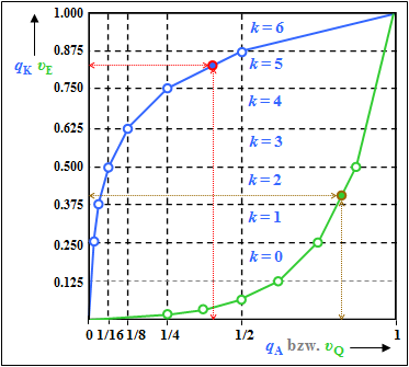
- In the compressor: $q_{\rm A} = 0.4$ led to the initial value $q_{\rm K} = 0.825$ and after quantization to the value $q_{\rm Q} = 0. 824$ ⇒ see subtasks (1) and (3). ⇒ red marks in the graph.
- On the receiver side, this results in $v_{\rm Q} = 0.824$ approximately back to $v_{\rm E} ≈ 0.4$ ⇒ brown marks in the graph.
- However, due to quantization, this is only an approximation. Exactly:
- $$ v_{\rm E} = 0.25 + \frac{0.824-0.750}{0.875-0.750} \cdot 0.25 \hspace{0.15cm}\underline {= 0.398} \hspace{0.05cm}.$$
This calculation process can be understood from the graph.
- Although the expander characteristic $v_E(υ_{\rm Q})$ is equal to the inverse function of the compressor characteristic $q_K(q_{\rm A})$ an error results because the input $v_{\rm Q}$ of the expander is discrete in value (influence of quantization).
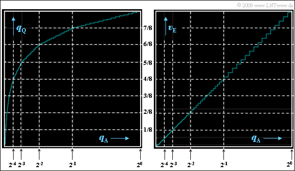
(6) Correct are the statements 1 and 4, as can be verified by the following left graph:
- The width of each step is different in each segment. In the outermost segment $(k = 6)$ the step width is $0.5/16 = 1/32$, in the next segment $(k = 5)$ only more $0.25/16 = 1/64$.
- The step widths in the further segments are $1/128 \ (k = 4)$, $1/256 \ (k = 3)$, $1/512\ (k = 2)$ and $1/1024 \ (k = 1)$.
- The innermost range from $-1/64$ to $+1/64$ is divided into $64$ steps, resulting in the step width $1/2048$.
- The step height, on the other hand, is constantly equal $1/8$ divided by $16 = 1/128$ in the segments $k ≠ 0$ and equal $1/256$ in the middle segment.
(7) Correct here is only the second statement:
- By the expander, the quantization is now along the bisector of the angle.
- In each segment, step width and step height are constant.
- As the right graphic shows, however, in the next inner segment the width and the height are only half as large.


