Difference between revisions of "Aufgaben:Exercise 3.3Z: Optimization of a Coaxial Cable System"
From LNTwww
| Line 23: | Line 23: | ||
''Notes:'' | ''Notes:'' | ||
| − | *The exercise belongs to the chapter [[Digital_Signal_Transmission/Consideration_of_Channel_Distortion_and_Equalization|Consideration of Channel Distortion and Equalization]]. | + | *The exercise belongs to the chapter [[Digital_Signal_Transmission/Consideration_of_Channel_Distortion_and_Equalization|"Consideration of Channel Distortion and Equalization"]]. |
| − | * Use the interaction module [[Applets:Komplementäre_Gaußsche_Fehlerfunktionen|Complementary Gaussian Error Functions]] for numerical evaluation of the Q-function.. | + | * Use the interaction module [[Applets:Komplementäre_Gaußsche_Fehlerfunktionen|"Complementary Gaussian Error Functions"]] for numerical evaluation of the Q-function.. |
Revision as of 16:56, 16 May 2022
We consider a redundancy-free binary transmission system with the following specifications:
- The transmission pulses are NRZ rectangular and have energy $E_{\rm B} = s_0^2 \cdot T$.
- The channel is a coaxial cable with characteristic cable attenuation $a_* = 40 \, {\rm dB}$.
- AWGN noise with noise power density $N_0 = 0.0001 \cdot E_{\rm B}$ is present.
- The receiver frequency response $H_{\rm E}(f)$ includes an ideal channel equalizer $H_{\rm K}^{\rm -1}(f)$ and a Gaussian low-pass filter $H_{\rm G}(f)$ with cutoff frequency $f_{\rm G}$ for noise power limitation.
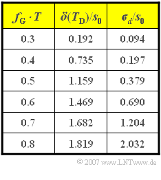
The table shows the eye opening $\ddot{o}(T_{\rm D})$ as well as the detection noise rms value $\sigma_{\rm d}$ – each normalized to the transmitted amplitude $s_0$ – for different cutoff frequencies $f_{\rm G}$. The cutoff frequency is to be chosen such that the worst-case error probability is as small as possible, with the following definition:
- $$p_{\rm U} = {\rm Q} \left( \frac{\ddot{o}(T_{\rm D})/2}{ \sigma_d} \right) \hspace{0.3cm}\Rightarrow \hspace{0.3cm} p_{\rm U} = {\rm Q} \left( \sqrt{\rho_{\rm U}}\right)$$
- This quantity represents an upper bound for the mean error probability $p_{\rm S}$: $p_{\rm S} \le p_{\rm U}$.
- For $f_{\rm G} \cdot T ≥ 0.4$, a lower bound can also be given: $p_{\rm S} \ge p_{\rm U}/4$.
Notes:
- The exercise belongs to the chapter "Consideration of Channel Distortion and Equalization".
- Use the interaction module "Complementary Gaussian Error Functions" for numerical evaluation of the Q-function..
Questions
Solution
(1) For the optimization it is sufficient to maximize the quotient $\ddot{o}(T_{\rm D})/\sigma_d$:
- This is maximized from the values given in the table for the cutoff frequency $f_{\rm G, opt} \cdot T \underline {= 0.4}$ with $0.735/0.197 \approx 3.73$.
- As a comparison: For $f_{\rm G} \cdot T = 0.3$ the result is $0.192/0.094 \approx 2.04$ due to the smaller eye opening and for $f_{\rm G} \cdot T = 0.5$ the quotient is also smaller than for the optimum: $1.159/0.379 \approx 3.05$.
- An even larger cutoff frequency leads to a very large noise rms value without simultaneously increasing the vertical eye opening in the same way.
(2) Using the result from (1), we further obtain:
- $$\rho_{\rm U} = \left ( {3.73}/{2} \right )^2 \approx 3.48 \hspace{0.3cm}\Rightarrow \hspace{0.3cm} 10 \cdot {\rm lg}\hspace{0.1cm}\rho_{\rm U} \hspace{0.15cm}\underline { = 5.41\,{\rm dB}}\hspace{0.3cm} \Rightarrow \hspace{0.3cm} p_{\rm U} = {\rm Q}\left ( {3.73}/{2} \right) \hspace{0.15cm}\underline {\approx 0.031} \hspace{0.05cm}.$$
(3)
- With the given $10 \cdot {\rm lg} \, E_{\rm B}/N_0 = 40 \ \rm dB$, i.e. $E_{\rm B}/N_0 = 10^4$, the worst-case signal-to-noise ratio has been found to be $10 \cdot {\rm lg} \, \rho_{\rm U} \approx 5.41 \, {\rm dB}$.
- However, for the worst-case error probability $p_{\rm U} = 10^{\rm -6}$, $10 \cdot {\rm lg} \, \rho_{\rm U} > 13.55 \, {\rm dB}$ must be obtained.
- This is achieved by increasing the quotient $E_{\rm B}/N_0$ accordingly:
- $$10 \cdot {\rm lg}\hspace{0.1cm}{E_{\rm B}}/{N_0} = 40\,{\rm dB} \hspace{0.1cm}+\hspace{0.1cm}13.55\,{\rm dB} \hspace{0.1cm}-\hspace{0.1cm}5.41\,{\rm dB}= 48.14\,{\rm dB}\hspace{0.3cm} \Rightarrow \hspace{0.3cm} {E_{\rm B}}/{N_0} = 10^{4.814}\approx 65163 \hspace{0.3cm}\Rightarrow \hspace{0.3cm} {N_0}/{E_{\rm B}}\hspace{0.15cm}\underline { = 1.53 \cdot 10^{-5}} \hspace{0.05cm}.$$
(4)
- The upper bound for $p_{\rm S}$ is equal to the worst-case error probability $p_{\rm U} = \underline {10^{\rm -6}}$.
- The lower bound is $\underline {0.25 \cdot 10^{\rm -6}}$, which is smaller by a factor of 4.
