Difference between revisions of "Aufgaben:Exercise 4.17Z: Rayleigh and Rice Distribution"
| Line 2: | Line 2: | ||
{{quiz-Header|Buchseite=Digital_Signal_Transmission/Carrier_Frequency_Systems_with_Non-Coherent_Demodulation}} | {{quiz-Header|Buchseite=Digital_Signal_Transmission/Carrier_Frequency_Systems_with_Non-Coherent_Demodulation}} | ||
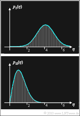
| − | [[File: | + | [[File:P_ID2079__Dig_Z_4_17_ret.png|right|frame|Rice (top) and Rayleigh (bottom)]] |
For the study of transmission systems, the Rayleigh and Rice distributions are of great importance. In the following let $y$ be a Rayleigh or a Rice distributed random variable and $\eta$ in each case a realization of it. | For the study of transmission systems, the Rayleigh and Rice distributions are of great importance. In the following let $y$ be a Rayleigh or a Rice distributed random variable and $\eta$ in each case a realization of it. | ||
* The "Rayleigh distribution" results thereby for the probability density function $\rm (PDF)$ of a random variable $y$, which results from the two Gaussian distributed and statistically independent components $u$ and $v$ $($both with the standard deviation $\sigma_n)$ as follows: | * The "Rayleigh distribution" results thereby for the probability density function $\rm (PDF)$ of a random variable $y$, which results from the two Gaussian distributed and statistically independent components $u$ and $v$ $($both with the standard deviation $\sigma_n)$ as follows: | ||
Latest revision as of 13:41, 10 October 2022
For the study of transmission systems, the Rayleigh and Rice distributions are of great importance. In the following let $y$ be a Rayleigh or a Rice distributed random variable and $\eta$ in each case a realization of it.
- The "Rayleigh distribution" results thereby for the probability density function $\rm (PDF)$ of a random variable $y$, which results from the two Gaussian distributed and statistically independent components $u$ and $v$ $($both with the standard deviation $\sigma_n)$ as follows:
- $$y = \sqrt{u^2 + v^2} \hspace{0.1cm} \Rightarrow \hspace{0.1cm} p_y (\eta) = \frac{\eta}{\sigma_n^2} \cdot {\rm exp } \left [ - \frac{\eta^2}{2 \sigma_n^2}\right ] \hspace{0.01cm}.$$
- The "Rice distribution" is obtained under otherwise identical boundary conditions for the application case where a constant $C$ is still added to one of the two components, for example:
- $$y = \sqrt{(u+C)^2 + v^2} \hspace{0.3cm} \Rightarrow \hspace{0.3cm} p_y (\eta) = \frac{\eta}{\sigma_n^2} \cdot {\rm exp } \left [ - \frac{\eta^2 + C^2}{2 \sigma_n^2}\right ] \cdot {\rm I }_0 \left [ \frac{\eta \cdot C}{ \sigma_n^2}\right ] \hspace{0.05cm}.$$
In this equation, ${\rm I}_0(x)$ denotes the "modified zero-order Bessel function".
In the graph, the two probability density functions are shown, but it is not indicated whether $p_{\hspace{0.03cm}\rm I}(\eta)$ or $p_{\hspace{0.03cm}\rm II}(\eta)$ belong to a Rayleigh or a Rice distribution, respectively.
- It is only known that one Rayleigh and one Rice distribution is shown.
- The parameter $\sigma_n$ is the same for both distributions.
For your decision whether to assign $p_{\hspace{0.03cm}\rm I}(\eta)$ or $p_{\rm II}(\hspace{0.03cm}\eta)$ to the Rice distribution and for the determination of the PDF parameters you can consider the following statements:
- For large values of the quotient $C/\sigma_n$, the Rice distribution can be approximated by a Gaussian distribution with mean $C$ and standard deviation $\sigma_n$.
- The values of $C$ and $\sigma_n$ underlying the graph are integers.
Regarding the Rayleigh distribution, note:
- The same $\sigma_n$ is used for both distributions.
- For the standard deviation (root of the variance) of the Rayleigh distribution holds:
- $$\sigma_y = \sigma_n \cdot \sqrt{2 - {\pi}/{2 }} \hspace{0.2cm} \approx \hspace{0.2cm} 0.655 \cdot \sigma_n \hspace{0.05cm}.$$
- For the standard deviation or for the variance of the Rice distribution in general only a complicated expression with hypergeometric functions can be given, otherwise only an approximation for $C \gg \sigma_n$ corresponding to the Gaussian distribution.
Notes:
- This exercise belongs to the chapter "Carrier Frequency Systems with Non-Coherent Demodulation".
- Given is also the following indefinite integral:
- $$\int x \cdot {\rm e }^{-x^2} \,{\rm d} x = -{1}/{2} \cdot {\rm e }^{-x^2} + {\rm const. } $$
Questions
Solution
- The upper graph shows approximately a Gaussian distribution and belongs accordingly to the Rice distribution.
(2) You can see from the graph: The mean value of the Gaussian distribution is $\underline {C = 4}$ and the standard deviation is $\underline {\sigma_n = 1}$.
- It was given that $C$ and $\sigma_n$ were integers. Thus the two density functions are:
- $$p_{\rm I} (\eta) \hspace{-0.1cm} \ = \ \hspace{-0.1cm} {\eta} \cdot {\rm exp } \left [ - \frac{\eta^2 + 16}{2 }\right ] \cdot {\rm I }_0 (4\eta ) \approx \frac{1}{\sqrt{2\pi }}\cdot {\rm exp } \left [ - \frac{(\eta-4)^2 }{2 }\right ]\hspace{0.05cm},$$
- $$ p_{\rm II} (\eta) \hspace{-0.1cm} \ = \ \hspace{-0.1cm} {\eta} \cdot {\rm exp } \left [ - \frac{\eta^2 }{2 }\right ] \hspace{0.05cm}.$$
(3) Solution 2 is correct, as can already be seen from the graph. A calculation confirms this result:
- $$\sigma_{\rm Rice}^2 \hspace{-0.1cm} \ = \ \hspace{-0.1cm} \sigma_n^2 = 1\hspace{0.05cm},$$
- $$ \sigma_{\rm Rayl}^2 \hspace{-0.1cm} \ = \ \hspace{-0.1cm} \sigma_n^2 \cdot ({2 - {\pi}/{2 }}) \approx 0.429 \hspace{0.05cm}.$$
(4) In general, the probability that $y$ is greater than a certain value $y_0$ is equal to
- $${\rm Pr}(y > y_0) = \int_{y_0}^{\infty} \frac{\eta}{\sigma_n^2} \cdot {\rm exp } \left [ - \frac{\eta^2 }{2 \sigma_n^2}\right ] \,{\rm d} \eta \hspace{0.05cm}.$$
- With the substitution $x^2 = \eta^2/(2\sigma_n^2)$ can be written for this:
- $${\rm Pr}(y > y_0) = 2 \cdot \hspace{-0.05cm}\int_{y_0/(\sqrt{2}\hspace{0.03cm} \cdot \hspace{0.03cm} \sigma_n)}^{\infty} \hspace{-0.5cm}x \cdot {\rm e }^{ - x^2} \,{\rm d} x = \left [{\rm e }^{ - x^2} \right ]_{\sqrt{2}\hspace{0.03cm} \cdot \hspace{0.03cm} \sigma_n}^{\infty} = {\rm exp } \left [ -\frac{ y_0^2 }{2 \sigma_n^2 }\right ]\hspace{0.05cm}.$$
- Here the indefinite integral given in the front was used. In particular:
- $${\rm Pr}(y > \sigma_n) \hspace{-0.1cm} \ = \ \hspace{-0.1cm} {\rm e }^{ - 0.5} \hspace{0.15cm} \underline{\approx 60.7 \%} \hspace{0.05cm},$$
- $$ {\rm Pr}(y > 2\sigma_n) \hspace{-0.1cm} \ = \ \hspace{-0.1cm} {\rm e }^{ - 2.0} \hspace{0.15cm} \underline{\approx 13.5 \%} \hspace{0.05cm},$$
- $$ {\rm Pr}(y > 3\sigma_n) \hspace{-0.1cm} \ = \ \hspace{-0.1cm} {\rm e }^{ - 4.5} \hspace{0.15cm} \underline{\approx 1.1 \%} \hspace{0.05cm}.$$
