Aufgaben:Exercise 3.9Z: Convolution of Gaussian Pulses

• Return to book

Gaussian pulses  $x(t)$,   $h(t)$

The convolution result of two Gaussian functions is to be determined.  We consider

• a Gaussian input pulse  ${x(t)}$  with amplitude $x_0 = 1\,\text{V}$ and  "equivalent pulse duration"  $\Delta t_x = 4 \,\text{ms}$,  as well as
• a likewise Gaussian impulse response  ${h(t)}$, which has the  "equivalent pulse duration"  $\Delta t_h = 3 \,\text{ms}$ :

$$x( t ) = x_0 \cdot {\rm{e}}^{ - {\rm{\pi }}( {t/\Delta t_x } )^2 } ,$$

$$h( t ) = \frac{1}{\Delta t_h } \cdot {\rm{e}}^{ - {\rm{\pi }}( {t/\Delta t_h } )^2 } .$$

The output signal  ${y(t)} = {x(t)} ∗{h(t)}$  is sought, whereby the diversions via the spectral functions is to be taken.

Hint:

• This exercise belongs to the chapter  The Convolution Theorem and Operation.

Questions

1 Give the spectral functions  ${X(f)}$  and  ${H(f)}$  an.  Which values result for  $f = 0$?

$X(f = 0)\ = \ $  $\text{mV/Hz}$

$H(f = 0)\ = \ $

2 Calculate the spectral function  ${Y(f)}$  of the output signal.  What is the spectral value at  $f = 0$?

$Y(f = 0)\ = \ $  $\text{mV/Hz}$

3 Calculate the output pulse  ${y(t)}$.  What values result for the amplitude  $y_0 = y(t = 0)$  and the equivalent pulse duration  $\Delta t_y$?

$y_0\ = \ $  $\text{V}$

$\Delta t_y\ = \ $  $\text{ms}$

Solution

Solution

(1)  By Fourier transformation one obtains:

$$X( f ) = x_0 \cdot \Delta t_x \cdot {\rm{e}}^{ - {\rm{\pi }}\left( {\Delta t_x \hspace{0.05cm}\cdot \hspace{0.05cm} f} \right)^2 } , \hspace{0.5cm}H(f) = {\rm{e}}^{ - {\rm{\pi }}\left( {\Delta t_h \hspace{0.05cm}\cdot \hspace{0.05cm}f} \right)^2 } .$$

• The values we are looking for are

$$X(f = 0)\;\underline{ = 4 \,\text{mV/Hz}}, \hspace{0.5cm}H(f = 0)\; \underline{= 1}.$$

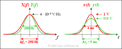
Gaussian spektra  $X(f)$,     $Y(f)$     –     Gaussian pulses  $x(t)$,     $y(t)$

(2)  Convolution in time domain corresponds to multiplication in frequency domain:

$$Y(f) = X(f) \cdot H(f) = x_0 \cdot \Delta t_x \cdot {\rm{e}}^{ - {\rm{\pi }}\left( {\Delta t_x^2 + \Delta t_h^2 } \right)f^2 } .$$

• With the abbreviation  $\Delta t_y = (\Delta t_x^2 + \Delta t_h^2)^{1/2} = 5\, \text{ms}$  one can write for this:

$$Y(f) = x_0 \cdot \Delta t_x \cdot {\rm{e}}^{ - {\rm{\pi }}\left( {\Delta t_y \hspace{0.05cm}\cdot \hspace{0.05cm} f} \right)^2 } .$$

• At frequency  $f = 0$ , the spectral values at the input and output of the Gaussian filter are equal, so:

$$Y(f = 0) \;\underline{= 4 \text{ mV/Hz}}.$$

• The function curve of  ${Y(f)}$  is narrower than  ${X(f)}$  and narrower than  ${H(f)}$.

(3)  The following Fourier correspondence holds:

$${\rm{e}}^{ - {\rm{\pi }}\left( {\Delta t_y \hspace{0.05cm}\cdot \hspace{0.05cm} f} \right)^2 }\bullet\!\!\!-\!\!\!-\!\!\!-\!\!\circ\, \frac{1}{\Delta t_y } \cdot {\rm{e}}^{ - {\rm{\pi }}\left( {t/\Delta t_y } \right)^2 } .$$

• This gives:

$$y(t) = x(t) * h(t) = x_0 \cdot \frac{\Delta t_x }{\Delta t_y } \cdot {\rm{e}}^{ - {\rm{\pi }}\left( {t/\Delta t_y } \right)^2 } .$$

• The maximum value of the signal  ${y(t)}$  is also at   $t = 0$  and is   $y_0 \hspace{0.15cm}\underline{= 0.8 \text{ V} }$.
• The equivalent pulse duration results in  $\Delta t_y \hspace{0.15cm}\underline{= 5 \text{ ms}}$  (see above graphic, right sketch).
• This means:  The Gaussian  ${H(f)}$  causes the output pulse  ${y(t)}$  to be smaller and wider than the input pulse  ${x(t)}$ .
• The pulse shape remains Gaussian.   Because:   Gaussian convoluted with Gaussian always results in Gaussian!