[[File:P_ID619__Sto_A_3_4.png|right|frame|Rechteck–WDF und Trapez–WDF]]
[[File:P_ID619__Sto_A_3_4.png|right|frame|Rectangular and trapezoidal PDF]]
Gegeben seien hier die drei Zufallsgrößen $x$, $y$ und $z$ , meist durch ihre jeweiligen Wahrscheinlichkeitsdichtefunktionen:
Given here are three random variables $x$, $y$ and $z$, mostly by their respective probability density functions:
*Über die Zufallsgröße $x$ ist nichts weiter bekannt: Diese kann sowohl eine diskrete als auch eine kontinuierliche Zufallsgröße sein und eine beliebige WDF $f_x(x)$ besitzen. Der Mittelwert ist allgemein gleich $m_x$.
*Nothing else is known about the random variable $x$: This can be both a discrete or a continuous random variable, and can have any PDF $f_x(x)$ The mean is generally equal $m_x$.
*Die kontinuierliche Zufallsgröße $y$ kann nur Werte im Bereich zwischen $1$ bis $3$ mit gleicher Wahrscheinlichkeit annehmen. Der Mittelwert ist $$m_y = 2.$$
*The continuous random variable $y$ can take values in the range between $1$ to $3$ with equal probability. Mean: $m_y = 2.$
*Die Zufallsgröße $z$ besitzt die folgende charakteristische Funktion:
*The random variable $z$ has the following characteristic function:
:Daneben wird noch der qualitative Verlauf der WDF $f_z(z)$ entsprechend der blauen Skizze als bekannt vorausgesetzt. Zu bestimmen sind die WDF-Parameter $a$, $b$ und $c$ dieser WDF.
:Besides, the qualitative course of the WDF $f_z(z)$ according to the blue sketch is assumed to be known. To be determined are the PDF parameters $a$, $b$, $c$ of this PDF.
Hints:
*This exercise belongs to the chapter [[Theory_of_Stochastic_Signals/Expected_Values_and_Moments|Expected values and moments]].
*Reference is made to the section [[Theory_of_Stochastic_Signals/Expected_Values_and_Moments#Characteristic_function|Charakteristic funcion]] .
''Hinweise:''
*Die Aufgabe gehört zum Kapitel [[Theory_of_Stochastic_Signals/Erwartungswerte_und_Momente|Erwartungswerte und Momente]].
*Insbesondere wird auf die Seite [[Theory_of_Stochastic_Signals/Erwartungswerte_und_Momente#Charakteristische_Funktion|Charakteristische Funktion]] Bezug genommen.
{Welche Aussagen sind bezüglich der charakteristischen Funktion $C_x ( {\it \Omega} )$ stets – also bei beliebiger WDF – gültig?
{Which statements are valid with respect to the characteristic function $C_x ( {\it \Omega} )$ always – that is, at any PDF ?
|type="[]"}
|type="[]"}
- $C_x ( {\it \Omega} )$ ist die Fouriertransformierte von $f_x(x)$.
- $C_x ( {\it \Omega} )$ is the Fourier transform of $f_x(x)$.
+ Der Realteil von $C_x ( {\it \Omega} )$ ist eine gerade Funktion in ${\it \Omega}$.
+ The real part of $C_x ( {\it \Omega} )$ is an even function in ${\it \Omega}$.
+ Der Imaginärteil von $C_x ( {\it \Omega} )$ ist eine ungerade Funktion in ${\it \Omega}$.
+ The imaginary part of $C_x ( {\it \Omega} )$ is an odd function in ${\it \Omega}$.
+ Der Wert an der Stelle ${\it \Omega} = 0$ ist stets $C_x ( {\it \Omega} ) = 1$.
+ The value at location ${\it \Omega} = 0$ is always $C_x ( {\it \Omega} ) = 1$.
- For a zero mean random variable $(m_x = 0)$ ⇒ $C_x ( {\it \Omega} )$ is always real.
{Berechnen Sie die charakteristische Funktion $C_y( {\it \Omega} )$. Wie groß sind Real- und Imaginärteil bei ${\it \Omega} = \pi/2$?
{Calculate the characteristic function $C_y( {\it \Omega} )$. What are the real and imaginary parts at ${\it \Omega} = \pi/2$?
*Die letzte Alternative trifft nicht immer zu: Eine zweipunktverteilte Zufallsgröße $x \in \{-1, +3\}$ mit den Wahrscheinlichkeiten $0.75$ und $0.25$ ist zwar mittelwertfrei $(m_x = 0)$, besitzt aber trotzdem eine komplexe charakteristische Funktion.
*The last alternative does not always hold: A two-point distributed random variable $x \in \{-1, +3\}$ with probabilities $0.75$ and $0.25$ is zero mean $(m_x = 0)$, but has still a complex characteristic function.
'''(2)''' Entsprechend der allgemeinen Definition gilt:
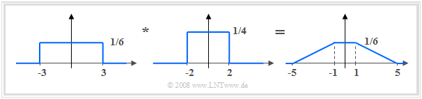
'''(3)''' Aus der angegebenen Korrespondenz kann abgelesen werden, dass ${\rm si}(3 {\it \Omega} )$ auf eine zwischen $\pm 3$ gleichverteilte Zufallsgröße zurückgeht und ${\rm si}(2 {\it \Omega} )$ die Transformierte einer Gleichverteilung zwischen $\pm 2$ angibt.
*In der charakteristischen Funktion sind diese beiden Anteile multiplikativ verknüpft. Damit ist die resultierende WDF $f_z(z)$ die Faltung dieser beiden Rechteckfunktionen:
'''(3)''' From the given correspondence it can be read that ${\rm si}(3 {\it \Omega} )$ is due to an between $\pm 3$ equally distributed random variable and ${\rm si}(2 {\it \Omega} )$ gives the transform of a uniform distribution between $\pm 2$.
[[File:P_ID620__Sto_A_3_4_c_neu.png|center|frame|Konstruktion der Trapez-WDF]]
[[File:P_ID620__Sto_A_3_4_c_neu.png|right|frame|Construction of the trapezoidal PDF]]
*Die drei WDF-Parameter lauten somit:
*In the characteristic function, these two proportions are multiplicatively linked.
Given here are three random variables $x$, $y$ and $z$, mostly by their respective probability density functions:
Nothing else is known about the random variable $x$: This can be both a discrete or a continuous random variable, and can have any PDF $f_x(x)$ The mean is generally equal $m_x$.
The continuous random variable $y$ can take values in the range between $1$ to $3$ with equal probability. Mean: $m_y = 2.$
The random variable $z$ has the following characteristic function:
Besides, the qualitative course of the WDF $f_z(z)$ according to the blue sketch is assumed to be known. To be determined are the PDF parameters $a$, $b$, $c$ of this PDF.
The last alternative does not always hold: A two-point distributed random variable $x \in \{-1, +3\}$ with probabilities $0.75$ and $0.25$ is zero mean $(m_x = 0)$, but has still a complex characteristic function.
(3) From the given correspondence it can be read that ${\rm si}(3 {\it \Omega} )$ is due to an between $\pm 3$ equally distributed random variable and ${\rm si}(2 {\it \Omega} )$ gives the transform of a uniform distribution between $\pm 2$.
Construction of the trapezoidal PDF
In the characteristic function, these two proportions are multiplicatively linked.
Thus, the resulting PDF $f_z(z)$ is the convolution of these two rectangular functions.