[[File:P_ID503__Sig_A_3_3.png|250px|right|Rechteckimpuls und Spektrum]]
[[File:EN_Sig_A_3_3.png|250px|right|frame|Rectangular pulse and its spectrum]]
Betrachtet wird ein Rechteckimpuls $x(t)$ der Dauer $T = 50\,\text{µs}$ und der Höhe $A = 2\,\text{V}$. An den Sprungstellen bei $t = 0$ und $t = T$ ist der Signalwert jeweils $A/2$, was aber für die Lösung der Aufgabe keinen Einfluss hat.
A rectangular pulse $x(t)$ with duration $T = 50\,\text{µs}$ and height $A = 2\,\text{V}$ is considered. At the jumping points at $t = 0$ and $t = T$ the signal value is $A/2$ in each case, but this has no influence on the solution of the task.
In der unteren Grafik ist die dazugehörige Spektralfunktion nach Betrag und Phase qualitativ skizziert. Es gilt:
In the lower graph, the corresponding spectral function is sketched qualitatively according to magnitude and phase. It is valid:
$$X( f ) = \left| {X( f )} \right| \cdot {\rm e}^{ - {\rm j}\hspace{0.05cm}\cdot \hspace{0.05cm} \varphi ( f )} .$$
:$$X( f ) = \left| {X( f )} \right| \cdot {\rm e}^{ - {\rm j}\hspace{0.05cm}\cdot \hspace{0.05cm} \varphi ( f )} .$$
Der analytische Funktionsverlauf von $X(f)$ soll ermittelt werden.
The analytical function progression of $X(f)$ is to be determined.
''Hinweise:''
*Die Aufgabe gehört zum Kapitel [[Signaldarstellung/Einige_Sonderfälle_impulsartiger_Signale|Einige Sonderfälle impulsartiger Signale]].
*Sollte die Eingabe des Zahlenwertes „0” erforderlich sein, so geben Sie bitte „0.” ein.
*Gegeben sind weiterhin folgende trigonometrischen Umformungen:
{Berechnen Sie die Betragsfunktion $|X(f)|$ allgemein. Welche Werte ergeben sich für die Frequenzen $f = 0$ und $f=20 \,\text{kHz})$?
{Calculate the magnitude function $|X(f)|$ in general. What values result for the frequencies $f = 0$ and $f=20 \,\text{kHz}$?
Bei der Berechnung des Spektralwertes für $f = 0$ erscheint der Quotient „0 durch 0”. Durch Anwendung der [https://de.wikipedia.org/wiki/Regel_von_de_l%E2%80%99Hospital Regel von l'Hospital] kann dieser Grenzwert berechnet werden:
*When calculating the value for $f = 0$ the quotient is $\text{"0 divided by 0"}$. By applying [https://en.wikipedia.org/wiki/L%27H%C3%B4pital%27s_rule L'Hospitals rule] the limiting value can be calculated:
$$\left| {X( {f = 0} )} \right| = A \cdot T \hspace{0.15 cm}\underline{= 0.1 \;{\rm{mV/Hz}}}{\rm{.}}$$
:$$\left| {X( {f = 0} )} \right| = A \cdot T \hspace{0.15 cm}\underline{= 0.1 \;{\rm{mV/Hz}}}{\rm{.}}$$
Dieses Ergebnis ist einsichtig, da nach dem ersten Fourierintegral der Spektralwert bei $f = 0$ genau der Fläche unter der Zeitfunktion entspricht.
*This result is obvious because, according to the first Fourier integral, the spectral value at $f = 0$ corresponds exactly to the area under the time function.
[[File:P_ID563__Sig_A_3_3_c.png|right|Betragsspektrum des Rechteckimpulses]]
'''3.''' Richtig sind somit die <u>Lösungsvorschläge 1 und 3</u>:
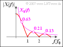
[[File:P_ID563__Sig_A_3_3_c.png|right|frame|Magnitude spectrum of the rectangular pulse]]
*Entsprechend dem Ergebnis zur Teilaufgabe (2) treten die Nullstellen im Abstand $f_0 = 1/T$ auf. Bei $f_0 = 1/(2T) = f = 10 \;{\rm{kHz}}$ ist zwar der Realteil $0$, aber nicht der Imaginärteil.
'''(3)''' The <u>proposed solutions 1 and 3</u> are correct:
*Bei den Argumenten $f \cdot T = 0.5, 1.5, 2.5, ... $ ist die Sinusfunktion jeweils betragsmäßig gleich $1$, und es gilt:
*According to the result of subtask '''(2)''' the zeros occur at the distance $f_0 = 1/T$ .
*With $f_0 = 1/(2T) = f = 10 \;{\rm{kHz}}$ the real part is $0$, but not the imaginary part.
*With the arguments $f \cdot T = 0.5,\ 1.5,\ 2.5,\hspace{0.05cm}\text{...}$ the sine function is in each case equal in magnitude to $1$, and it holds:
:$$\left| {X( f )} \right| = \frac{A}{ {{\rm{\pi }}\left| f \right|}} = X_{\rm S} ( f ).$$
:$$\left| {X( f )} \right| = \frac{A}{ {{\rm{\pi }}\left| f \right|}} = X_{\rm S} ( f ).$$
Bei anderen Frequenzen dient $X_{\rm S}(f)$ als obere Schranke, d. h. es gilt stets ($|Xf)| \geq X_{\rm S}(f)$. In obiger Skizze ist diese Schranke zusätzlich zu $|X(f)|$ als violette Kurve eingezeichnet.
*At other frequencies, $X_{\rm S}(f)$ serves as an upper bound, i.e. $|Xf)| \leq X_{\rm S}(f)$ always applies.
*In the sketch, this bound is drawn as a violet curve in addition to $|X(f)|$.
'''4.''' Nach der Definition auf der Angabenseite kann man die Phasenfunktion wie folgt berechnen:
'''(4)''' According to the definition on the information page, one can calculate the phase function as follows:
$$\varphi ( f ) = - \arctan \frac{ { {\mathop{\rm Im}\nolimits} ( f )}}{ { {\mathop{\rm Re}\nolimits} ( f )}}.$$
:$$\varphi ( f ) = - \arctan \frac{ { {\mathop{\rm Im}\nolimits} ( f )}}{ { {\mathop{\rm Re}\nolimits} ( f )}}.$$
Mit den Ergebnissen aus Teilaufgabe (1) gilt somit:
*With the results from subtask '''(1)''' the following thus applies:
Das Argument dieser Funktion ist entsprechend der Angabe gleich $\tan(\omega T/2) = \tan(\pi fT)$. Daraus folgt ein mit der Frequenz linear ansteigender Verlauf:
*The argument of this function is equal to $\tan(\omega T/2) = \tan(\pi fT)$ according to the specification. From this follows a linearly increasing course with frequency:
A rectangular pulse $x(t)$ with duration $T = 50\,\text{µs}$ and height $A = 2\,\text{V}$ is considered. At the jumping points at $t = 0$ and $t = T$ the signal value is $A/2$ in each case, but this has no influence on the solution of the task.
In the lower graph, the corresponding spectral function is sketched qualitatively according to magnitude and phase. It is valid:
$$X( f ) = \left| {X( f )} \right| \cdot {\rm e}^{ - {\rm j}\hspace{0.05cm}\cdot \hspace{0.05cm} \varphi ( f )} .$$
The analytical function progression of $X(f)$ is to be determined.
$$\left| {X( {f = 0} )} \right| = A \cdot T \hspace{0.15 cm}\underline{= 0.1 \;{\rm{mV/Hz}}}{\rm{.}}$$
This result is obvious because, according to the first Fourier integral, the spectral value at $f = 0$ corresponds exactly to the area under the time function.
Magnitude spectrum of the rectangular pulse
(3) The proposed solutions 1 and 3 are correct:
According to the result of subtask (2) the zeros occur at the distance $f_0 = 1/T$ .
With $f_0 = 1/(2T) = f = 10 \;{\rm{kHz}}$ the real part is $0$, but not the imaginary part.
With the arguments $f \cdot T = 0.5,\ 1.5,\ 2.5,\hspace{0.05cm}\text{...}$ the sine function is in each case equal in magnitude to $1$, and it holds:
$$\left| {X( f )} \right| = \frac{A}{ {{\rm{\pi }}\left| f \right|}} = X_{\rm S} ( f ).$$
At other frequencies, $X_{\rm S}(f)$ serves as an upper bound, i.e. $|Xf)| \leq X_{\rm S}(f)$ always applies.
In the sketch, this bound is drawn as a violet curve in addition to $|X(f)|$.
(4) According to the definition on the information page, one can calculate the phase function as follows:
$$\varphi ( f ) = - \arctan \frac{ { {\mathop{\rm Im}\nolimits} ( f )}}{ { {\mathop{\rm Re}\nolimits} ( f )}}.$$
With the results from subtask (1) the following thus applies:
The argument of this function is equal to $\tan(\omega T/2) = \tan(\pi fT)$ according to the specification. From this follows a linearly increasing course with frequency: