Aufgaben:Exercise 4.14Z: Echo Detection: Difference between revisions

From LNTwww
Nabil (talk | contribs)
Die Seite wurde neu angelegt: „ {{quiz-Header|Buchseite=Stochastische Signaltheorie/Kreuzkorrelationsfunktion und Kreuzleistungsdichte }} right| :Zur Messu…“
 
Fix interlanguage link: resolve redirect chain
 
(30 intermediate revisions by 6 users not shown)
Line 1: Line 1:


{{quiz-Header|Buchseite=Stochastische Signaltheorie/Kreuzkorrelationsfunktion und Kreuzleistungsdichte
{{quiz-Header|Buchseite=Theory_of_Stochastic_Signals/Cross-Correlation_Function_and_Cross_Power_Density
}}
}}


[[File:P_ID440__Sto_Z_4_14.png|right|]]
[[File:EN_Sto_Z_4_14.png|right|Echo measuring arrangement|frame]]
:Zur Messung akustischer Echos in R&auml;umen &ndash; zum Beispiel bedingt durch Reflexionen an einer Wand &ndash; kann die nebenstehende Anordnung verwendet werden. Der Rauschgenerator erzeugt ein &bdquo;im relevanten Frequenzbereich Wei&szlig;es Rauschen&rdquo; <i>x</i>(<i>t</i>) mit der Rauschleistungsdichte <i>N</i><sub>0</sub> = 10<sup>&ndash;6</sup> W/Hz. Dieses ist bandbegrenzt auf <i>B<sub>x</sub></i> = 20 kHz und wird auf einen Lautsprecher gegeben. Die gesamte Messeinrichtung ist für den Widerstandswert <i>R</i> = 50 &Omega; ausgelegt.
To measure acoustic echoes in rooms&nbsp; &ndash; for example caused by reflections at a wall &ndash;&nbsp; the adjacent setup can be used:
*The noise generator produces a&nbsp; "white noise in the relevant frequency range"&nbsp; $x(t)$&nbsp; with power density&nbsp; $N_0 = 10^{-6} \hspace{0.08cm} \rm W/Hz$.  
*This is bandlimited to&nbsp; $B_x = 20 \hspace{0.08cm} \rm kHz$&nbsp; and is given to a loudspeaker.  
*The entire measurement setup is designed for the resistance value&nbsp; $R = 50 \hspace{0.08cm} \rm \Omega$.


:Das vom Mikrofon aufgenommene Signal ist im allgemeinsten Fall wie folgt beschreibbar:
 
In the most general case,&nbsp; the signal recorded by the microphone can be described as follows:
:$$y(t) = \sum_{\mu = 1}^M \alpha_\mu \cdot x ( t - t_\mu ) .$$


:Hierbei bezeichnen <i>&alpha;<sub>&mu;</sub></i> Dämpfungsfaktoren und <i>t<sub>&mu;</sub></i> Laufzeiten.
Here the&nbsp; $\alpha_\mu$&nbsp; denote damping factors and&nbsp; $t_\mu$&nbsp; delay times.


:Bei dem hier gezeichneten Zweiwegemodell gilt <i>M</i> = 2: Zu dem direkten Pfad <i>S</i><sub>1</sub> kommt hier der Umweg <i>S</i><sub>2</sub> hinzu. Benutzen Sie f&uuml;r numerische Berechnungen die Parameterwerte
:$$\alpha_1 = 0.5, \hspace{0.2cm}t_1 = 200 \,{\rm ms}, \hspace{0.2cm}, \alpha_2 = 0.1, \hspace{0.2cm}t_2 = 250 \,{\rm ms}.$$


:<b>Hinweis:</b> Diese Aufgabe bezieht sich auf den Lehrstoff von Kapitel 4.6.


===Fragebogen===
Hints:
*The exercise belongs to the chapter&nbsp; [[Theory_of_Stochastic_Signals/Cross-Correlation_Function_and_Cross_Power_Density|Cross-Correlation Function and Cross Power-Spectral Density]].
*Use for numerical calculations the parameter values.
:$$\alpha_1 = 0.5, \hspace{0.2cm}t_1 = 200 \,{\rm ms}, \hspace{0.2cm} \alpha_2 = 0.1, \hspace{0.2cm}t_2 = 250 \,{\rm ms}.$$


===Questions===


<quiz display=simple>
{Geben Sie die AKF <i>&phi;<sub>x</sub></i>(<i>&tau;</i>) am Sender an. Wie lautet diese umgerechnet auf den Widerstand R = 1 &Omega;? Wie gro&szlig; ist der Effektivwert <i>&sigma;<sub>x</sub></i>?
{Apply the&nbsp; $\rm ACF$&nbsp; $\varphi_x(\tau)$&nbsp; at the transmitter.&nbsp; What means this converted to the resistor&nbsp; $R = 50 \hspace{0.08cm} \rm \Omega$&nbsp;?&nbsp; What is the rms value&nbsp; $\sigma_x$&nbsp;?
|type="{}"}
|type="{}"}
$\sigma_x$ = { 1 3% } $V$
$\sigma_x \ = \ $ { 1 3% } $\ \rm V$


{Berechnen Sie die KKF <i>&phi;<sub>xy</sub></i>(<i>&tau;</i>) zwischen Sende&ndash; und Empfangssignal. Welche Werte ergeben sich f&uuml;r <i>&tau;</i> = 0, <i>&tau;</i> = <i>t</i><sub>1</sub> und <i>&tau;</i> = <i>t</i><sub>2</sub>?
{Calculate the cross-correlation function&nbsp; $\rm (CCF)$ &nbsp; $\varphi_{xy}(\tau)$&nbsp; between transmitted and received signal. <br>What values result for&nbsp; $\tau = 0$, &nbsp; $\tau = t_1 = 200 \hspace{0.08cm} \rm ms$ &nbsp; and &nbsp; $\tau = t_2 = 250 \hspace{0.08cm} \rm ms$&nbsp;?
|type="{}"}
|type="{}"}
<i>&phi;<sub>xy</sub></i>(<i>&tau; = 0</i>) = { 0 3% } $V^2$
$\varphi_{xy}(\tau= 0) \ = \ $ { 0. } $\ \rm V^2$
<i>&phi;<sub>xy</sub></i>(<i>&tau; = 200 ms</i>) = { 0.5 3% } $V^2$
$\varphi_{xy}(\tau= t_1) \ = \ $ { 0.5 3% } $\ \rm V^2$
<i>&phi;<sub>xy</sub></i>(<i>&tau; = 250 ms</i>) = { 0.1 3% } $V^2$
$\varphi_{xy}(\tau= t_2) \ = \ $ { 0.1 3% } $\ \rm V^2$


{Berechnen Sie das Kreuzleistungsdichtespektrum <i>&Phi;<sub>xy</sub></i>(<i>f</i>). Welcher Wert ergibt sich bei der Frequenz <i>f</i> = 0?
{Calculate the cross power-spectral density &nbsp; ${\it \Phi}_{xy}(f)$.&nbsp; What value is obtained at frequency $f = 0$?
|type="{}"}
|type="{}"}
$\phi_\text{xy}(f = 0)$ = { 15 3% } $.10^{-6}\ V^2/Hz$
${\it \Phi}_{xy}(f =0)\ = \ $ { 15 3% } $\ \cdot 10^{-6}\ \rm V^2\hspace{-0.1cm}/Hz$


{Welche der nachfolgenden Aussagen sind zutreffend, wenn Sie anstelle der in (a) berechneten AKF die N&auml;herung <i>&phi;<sub>x</sub></i>(<i>&tau;</i>) &asymp; <i>N</i><sub>0</sub>/2 &middot; &delta;(<i>&tau;</i>) verwenden?
{Which of the following statements are true if you use the approximation&nbsp; $\varphi_{x}(\tau) \approx N_0/2 \cdot \delta(\tau)$&nbsp; instead of the ACF calculated in&nbsp; '''(1)'''?
|type="[]"}
|type="[]"}
+ Das Rauschen ist nun &bdquo;echt&rdquo; wei&szlig; &ndash; also nicht bandbegrenzt.
+ The noise is now&nbsp; "true white"&nbsp; &ndash; so it is not bandlimited.
- Die Rauschleistung wird gegen&uuml;ber Punkt (1) vermindert.
- The noise power is reduced compared to subtask&nbsp; '''(1)'''.
+ Die KKF ist die Summe gewichteter und verschobener Diracs.
+ The cross-correlation function is the sum of weighted and shifted Dirac delta functions.
- Das Kreuzleistungsdichtespektrum ist wie unter (3) berechnet.
- The cross power-spectral density is calculated as in subtask&nbsp; '''(3)'''.


{Berechnen Sie unter Verwendung der N&auml;herung <i>&phi;<sub>x</sub></i>(<i>&tau;</i>) &asymp; <i>N</i><sub>0</sub>/2  &middot; &delta;(<i>&tau;</i>) die AKF  <i>&phi;<sub>y</sub></i>(<i>&tau;</i>). Welche Gewichte ergeben sich bei <i>&tau;</i> = 0 und <i>&tau;</i> = &Delta;<i>t</i> = <i>t</i><sub>2</sub> &ndash; <i>t</i><sub>1</sub>?
{Calculate the&nbsp; $\rm ACF$&nbsp; $\varphi_y(\tau)$&nbsp; using the approximation&nbsp; $\varphi_{xy}(\tau) \approx N_0/2 \cdot \delta(\tau)$.   &nbsp; What weights result for &nbsp; $\tau = 0$ &nbsp; and &nbsp; $\tau = \Delta t = t_2 - t_1$?
|type="{}"}
|type="{}"}
<i>&phi;<sub>y</sub></i>(<i>&tau; = 0</i>) = { 13 3% } $.10^{-8}\ W/hz$
$\varphi_{y}(\tau= 0) \ = \ $ { 0.13 3% } $\ \cdot 10^{-6}\ \rm W\hspace{-0.1cm}/Hz$
<i>&phi;<sub>y</sub></i>(<i>&tau; = &Delta; t</i>) = { 2.5 3% } $.10^{-8}\ W/hz$
$\varphi_{y}(\tau= \Delta t) \ = \ $ { 0.025 3% } $\ \cdot 10^{-6}\ \rm W\hspace{-0.1cm}/Hz$


</quiz>
</quiz>


===Musterlösung===
===Solution===
{{ML-Kopf}}
{{ML-Kopf}}
:<b>1.</b>&nbsp;&nbsp;Das zweiseitige Leistungsdichtespektrum <i>&Phi;<sub>x</sub></i>(<i>f</i>) ist im Bereich von -<i>B<sub>x</sub></i> bis <i>B<sub>x</sub></i> konstant gleich <i>N</i><sub>0</sub>/2. Dessen Fouriertransformierte ergibt die AKF:
'''(1)'''&nbsp; The two-sided power-spectral density&nbsp; ${\it \Phi}_{x}(f)$&nbsp; is constantly equal&nbsp; $N_0/2$&nbsp; in the range&nbsp; $\pm B_x$.  
:$$\varphi_x (\tau) = \frac{N_0}{2} \cdot 2 B_x \cdot {\rm si} (2 \pi B_x \tau) = 0.02 \hspace {0.05cm}{\rm W} \cdot {\rm si} (2 \pi B_x \tau).$$
*The Fourier transform is the ACF:
:$$\varphi_x (\tau) = {N_0}/{2} \cdot 2 B_x \cdot {\rm sinc} (2 B_x \tau) = 0.02 \hspace {0.08cm}{\rm W} \cdot {\rm sinc} (2 B_x \tau).$$
 
*Converted from &nbsp; $R = 50 \hspace{0.08cm} \rm \Omega$ &nbsp; to &nbsp; $R = 1 \hspace{0.08cm} \rm \Omega$ &nbsp; one obtains&nbsp; $($multiplication by&nbsp; $R = 50 \hspace{0.08cm} \rm \Omega)$:
:$$\varphi_x (\tau) = 0.02 \hspace {0.05cm}{\rm VA} \cdot 50 \hspace {0.05cm}{\rm V/A}\cdot {\rm sinc} (2 B_x \tau)= 1 \hspace {0.05cm}{\rm V}^2 \cdot {\rm sinc} (2 B_x \tau).$$


:Umgerechnet von <i>R</i> = 50 &Omega; auf <i>R</i> = 1 &Omega; erh&auml;lt man somit (Multiplikation mit <i>R</i>  = 50 &Omega;):
*The rms value is the square root of the ACF value at&nbsp; $\tau = 0$: &nbsp;  
:$$\varphi_x (\tau) =  0.02 \hspace {0.05cm}{\rm VA} \cdot 50 \hspace {0.05cm}{\rm V/A}\cdot {\rm si} (2 \pi B_x \tau)= 1 \hspace {0.05cm}{\rm V}^2 \cdot {\rm si} (2 \pi B_x \tau).$$
:$$\sigma_x \hspace{0.15cm}\underline{= 1 \hspace {0.08cm}{\rm V}}.$$


:Der Effektivwert ist die Wurzel aus dem AKF-Wert bei <i>&tau;</i> = 0:
:$$\sigma_x \hspace{0.15cm}\underline{=  1 \hspace {0.05cm}{\rm V}}.$$


:<b>2.</b>&nbsp;&nbsp;F&uuml;r die KKF gilt im vorliegenden Fall:
'''(2)'''&nbsp; For the cross correlation function&nbsp; (CCF),&nbsp; in the present case:
:$$\varphi_{xy} (\tau) = \overline {x(t) \hspace{0.05cm}\cdot \hspace{0.05cm}y(t+\tau)} = \overline {x(t) \hspace{0.05cm}\cdot \hspace{0.05cm}\left [ \alpha_1 \cdot x(t- t_1+ \tau)\hspace{0.1cm}+\hspace{0.1cm} \alpha_2 \cdot x(t- t_2+ \tau)\right] } . $$
:$$\varphi_{xy} (\tau) = \overline {x(t) \hspace{0.05cm}\cdot \hspace{0.05cm}y(t+\tau)} = \overline {x(t) \hspace{0.05cm}\cdot \hspace{0.05cm}\big [ \alpha_1 \cdot x(t- t_1+ \tau)\hspace{0.1cm}+\hspace{0.1cm} \alpha_2 \cdot x(t- t_2+ \tau)\big] } . $$


:Nach Aufspaltung der Mittelwertbildung auf die beiden Terme erh&auml;lt man hieraus:
*After splitting the averaging on two terms,&nbsp; we get:
:$$\varphi_{xy} (\tau) = \alpha_1 \cdot \overline {x(t) \hspace{0.05cm}\cdot \hspace{0.05cm} x(t- t_1+ \tau)} \hspace{0.1cm}+\hspace{0.1cm} \alpha_2 \cdot \overline {x(t) \hspace{0.05cm}\cdot \hspace{0.05cm} x(t- t_2+ \tau)} .$$


:Unter Verwendung der AKF kann hierf&uuml;r auch geschrieben werden:
*Using the ACF&nbsp; $\varphi_x(\tau)$&nbsp; can also be written:
:$$\varphi_{xy} (\tau) = \alpha_1 \cdot {\varphi_{x}(\tau- t_1)} \hspace{0.1cm}+\hspace{0.1cm} \alpha_2\cdot {\varphi_{x}(\tau- t_2)} = \\ = 1 \hspace {0.05cm}{\rm V}^2 \cdot \left[ \alpha_1 \cdot {\rm si} (2 \pi B_x (\tau - t_1)) + \alpha_2 \cdot {\rm si} (2 \pi B_x (\tau - t_2))  \right].$$
:$$\varphi_{xy} (\tau) = \alpha_1 \cdot {\varphi_{x}(\tau- t_1)} \hspace{0.1cm}+\hspace{0.1cm} \alpha_2\cdot {\varphi_{x}(\tau- t_2)} = 1 \hspace {0.08cm}{\rm V}^2 \cdot \big[ \alpha_1 \cdot {\rm sinc} (2 B_x (\tau - t_1)) + \alpha_2 \cdot {\rm sinc} (2 B_x (\tau - t_2))  \big].$$
 
*The sinc&ndash;function exhibits equidistant zero crossings at all multiples of&nbsp; $1/(2B_x) = 25 \hspace{0.08cm} &micro; \rm s$,&nbsp; related to the centers at&nbsp; $t_1 = 200 \hspace{0.08cm} {\rm ms}$&nbsp; and&nbsp; $t_2 = 250 \hspace{0.08cm} {\rm ms}$.&nbsp; This results in the CCF values:
:$$\varphi_{xy} (\tau = 0) \hspace{0.15cm}\underline{= 0},\hspace{0.5cm}\varphi_{xy} (\tau = t_1)= \alpha_1 \cdot \varphi_{x} (\tau = 0) \hspace{0.15cm}\underline{= 0.5\,{\rm V}^2} ,\hspace{0.5cm} \varphi_{xy} (\tau = t_2)= \alpha_2 \cdot \varphi_{x} (\tau = 0) \hspace{0.15cm}\underline{= 0.1\,{\rm V}^2} .$$


:Die si-Funktion weist &auml;quidistante Nulldurchg&auml;nge bei allen Vielfachen von 1/(2<i>B<sub>x</sub></i>) = 25 &mu;s auf, jeweils bezogen auf  deren Mittellagen bei <i>t</i><sub>1</sub> = 200 ms bzw. <i>t</i><sub>2</sub> = 250 ms.
'''(3)'''&nbsp; The cross power-spectral density is the Fourier transform of the CCF,&nbsp; just as the power-spectral density&nbsp;$\rm  (PSD)$&nbsp; gives the Fourier transform of the ACF.&nbsp; It holds:
:$${\it \Phi}_{xy} (f) = \alpha_1 \cdot {\it \Phi}_{x} (f) \cdot {\rm e}^{-{\rm j}2 \pi f t_1} \hspace{0.15cm}+ \hspace{0.15cm}\alpha_2 \cdot {\it \Phi}_{x} (f) \cdot {\rm e}^{-{\rm j}2 \pi f t_2}. $$


:Daraus ergeben sich die KKF-Werte zu:
*Outside of the range&nbsp; $|f| \le B_x$&nbsp; the power-spectral density&nbsp; ${\it \Phi}_{x}(f)$&nbsp; &ndash; and correspondingly the cross power-spectral density&nbsp; ${\it \Phi}_{xy}(f)$ &ndash; is identically zero.
:$$\varphi_{xy} (\tau = 0) \hspace{0.15cm}\underline{= 0} ,$$
*In contrast,&nbsp; inside this interval holds&nbsp; ${\it \Phi}_{x}(f) = N_0/2$.&nbsp; It follows in this range:
:$$\varphi_{xy} (\tau = t_1)= \alpha_1 \cdot \varphi_{x} (\tau = 0) \hspace{0.15cm}\underline{= 0.5\,{\rm V}^2} ,$$
[[File:P_ID450__Sto_Z_4_14_d.png|right|frame|ACF and CCF with white noise]]
:$$\varphi_{xy} (\tau = t_2)= \alpha_2 \cdot \varphi_{x} (\tau = 0) \hspace{0.15cm}\underline{= 0.1\,{\rm V}^2} .$$
:$${\it \Phi}_{xy} (f) = {N_0}/{2} \left( \alpha_1 \cdot {\rm e}^{-{\rm j}2 \pi f t_1} \hspace{0.15cm}+ \hspace{0.15cm}\alpha_2 \cdot {\rm e}^{-{\rm j}2 \pi f t_2} \right). $$


:<b>3.</b>&nbsp;&nbsp;Das Kreuzleistungsdichtespektrum ist die Fouriertransformierte der KKF, ebenso wie das LDS die Fouriertransformierte der AKF angibt. Mit den Ergebnissen aus 2) und 3) gilt deshalb:
*It is evident that&nbsp; ${\it \Phi}_{xy}(f)$&nbsp; unlike&nbsp; ${\it \Phi}_{x}(f)$&nbsp; is a complex function.&nbsp; For&nbsp; $f = 0$&nbsp; holds:
:$${\it \Phi}_{xy} (f) = \alpha_1 \cdot {\it \Phi}_{x} (f) \cdot {\rm e}^{-{\rm j}2 \pi f t_1} \hspace{0.15cm}+ \hspace{0.15cm}\alpha_2 \cdot {\it \Phi}_{x} (f) \cdot {\rm e}^{-{\rm j}2 \pi f t_2}. $$
:$${\it \Phi}_{xy} (f = 0) = {N_0}/{2} \left( \alpha_1 \hspace{0.15cm}+ \hspace{0.15cm}\alpha_2 \right) = 0.3 \cdot 10^{-6}\hspace{0.05cm}{\rm W/Hz} \hspace{0.15cm}\underline{= 15 \cdot 10^{-6}\hspace{0.07cm}{\rm V^2/Hz}} . $$


:Au&szlig;erhalb des Bereichs |<i>f</i>| &#8804; <i>B<sub>x</sub></i> ist das LDS <i>&Phi;<sub>x</sub></i>(<i>f</i>) - und dementsprechend auch das KLDS <i>&Phi;<sub>xy</sub></i>(<i>f</i>) - identisch 0. Innerhalb dieses Intervalls gilt <i>&Phi;<sub>x</sub></i>(<i>f</i>) = <i>N</i><sub>0</sub>/2. Daraus folgt in diesem Bereich:
:$${\it \Phi}_{xy} (f) = \frac{N_0}{2} \left( \alpha_1 \cdot {\rm e}^{-{\rm j}2 \pi f t_1} \hspace{0.15cm}+  \hspace{0.15cm}\alpha_2 \cdot {\rm e}^{-{\rm j}2 \pi f t_2} \right). $$


:Es ist ersichtlich, dass <i>&Phi;<sub>xy</sub></i>(<i>f</i>) im Gegensatz zu <i>&Phi;<sub>x</sub></i>(<i>f</i>) eine komplexe Funktion ist. Bei <i>f</i> = 0 gilt:
:$${\it \Phi}_{xy} (f = 0) = \frac{N_0}{2} \left( \alpha_1 \hspace{0.15cm}+  \hspace{0.15cm}\alpha_2 \right) = 0.3 \cdot 10^{-6}\hspace{0.05cm}{\rm W/Hz} \hspace{0.15cm}\underline{= 15 \cdot 10^{-6}\hspace{0.07cm}{\rm V^2/Hz}} . $$
[[File:P_ID450__Sto_Z_4_14_d.png|right|]]


:<b>4.</b>&nbsp;&nbsp;Die Fouriertransformierte einer diracf&ouml;rmigen AKF f&uuml;hrt zu einem f&uuml;r alle Frequenzen <i>f</i> konstanten LDS, das hei&szlig;t tats&auml;chlich zu echt &bdquo;Wei&szlig;em Rauschen&rdquo;. Dieses besitzt eine unendlich gro&szlig;e Leistung, und f&uuml;r die KKF kann dann geschrieben werden:
'''(4)'''&nbsp; Correct are&nbsp; <u>the proposed solutions 1 and 3</u>:
:$$\varphi_{xy} (\tau) = \frac{\alpha_1 N_0}{2} \cdot {\rm \delta}( \tau - t_1) \hspace {0.1cm}+ \hspace {0.1cm}  \frac{\alpha_2  N_0}{2} \cdot {\rm \delta}( \tau - t_2) .$$
*The Fourier transform of a Dirac-shaped ACF leads to a constant PSD for all frequencies&nbsp; $f$ &nbsp; &rArr; &nbsp; "true white noise".  
*This has an infinitely large power,&nbsp; and for the CCF can then be written according to the above graph:
:$$\varphi_{xy} (\tau) = \alpha_1 \cdot { N_0}/{2} \cdot {\rm \delta}( \tau - t_1) \hspace {0.1cm}+ \hspace {0.1cm}  \alpha_2 \cdot { N_0}/{2} \cdot { \rm \delta}( \tau - t_2) .$$
*In the frequency domain,&nbsp; no difference is detectable for&nbsp; $|f| \le B_x$&nbsp; compared to subtask&nbsp; '''(3)'''&nbsp; .
*But since&nbsp; "true white noise"&nbsp; is now present,&nbsp; here the cross power-spectral density is not limited to this range.


:Dieser Verlauf ist in der Grafik oben skizziert.


:Im Frequenzbereich ist für |<i>f</i>| &#8804; <i>B<sub>x</sub></i> tats&auml;chlich kein Unterschied gegen&uuml;ber Teilaufgabe 3) feststellbar. Da nun aber echt wei&szlig;es Rauschen vorliegt, ist hier im Gegensatz zu Punkt c) das KLDS nicht auf diesen Bereich beschr&auml;nkt. Richtig sind demnach <u>die Lösungsvorschläge 1 und 3</u>.


:<b>5.</b>&nbsp;&nbsp;Die AKF des echobehafteten Signals lautet wie folgt:
'''(5)'''&nbsp; For the ACF of the echoed signal, &nbsp; $\varphi_{y} (\tau) = \overline {y(t) \hspace{0.05cm}\cdot \hspace{0.05cm}y(t+\tau)}$.
:$$\varphi_{y} (\tau) = \overline {y(t) \hspace{0.05cm}\cdot \hspace{0.05cm}y(t+\tau)} \\ \alpha_1^2 \hspace{0.02cm}\cdot\hspace{0.02cm} \overline {x(t - t_1) \hspace{0.02cm}\cdot \hspace{0.02cm}x(t - t_1+ \tau)} \hspace{0.1cm} + \hspace{0.1cm} \alpha_1\hspace{0.02cm}\cdot \hspace{0.02cm}\alpha_2 \hspace{0.02cm}\cdot\hspace{0.02cm} \overline {x(t - t_1) \hspace{0.02cm}\cdot \hspace{0.02cm}x(t - t_2+ \tau)} \\  + \hspace{0.05cm} \alpha_2\hspace{0.02cm}\cdot \hspace{0.02cm}\alpha_1 \hspace{0.02cm}\cdot\hspace{0.02cm} \overline {x(t - t_2) \hspace{0.02cm}\cdot \hspace{0.02cm}x(t - t_1+ \tau)}\hspace{0.1cm} + \hspace{0.1cm}\alpha_2^2 \hspace{0.02cm}\cdot\hspace{0.02cm} \overline {x(t - t_2) \hspace{0.02cm}\cdot \hspace{0.02cm}x(t - t_2+ \tau)}. $$
*This ACF&nbsp; $\varphi_{y} (\tau)$&nbsp; can consequently be represented as the following sum:
:$$\alpha_1^2 \cdot \overline {x(t - t_1) \cdot x(t - t_1+ \tau)} \hspace{0.03cm} + \hspace{0.03cm} \alpha_1\hspace{0.02cm}\alpha_2 \cdot \overline {x(t - t_1) \cdot x(t - t_2+ \tau)} + \hspace{0.05cm} \alpha_2\hspace{0.02cm}\alpha_1 \cdot \overline {x(t - t_2) \cdot x(t - t_1+ \tau)}\hspace{0.03cm} + \hspace{0.03cm} \alpha_2^2 \cdot \overline {x(t - t_2) \cdot x(t - t_2+ \tau)}. $$


:F&uuml;r den ersten und den letzten Mittelwert gilt:
*For the first and the last mean:
:$$\overline {x(t - t_1) \hspace{0.05cm}\cdot \hspace{0.05cm}x(t - t_1+ \tau)} = \overline {x(t - t_2) \hspace{0.05cm}\cdot \hspace{0.05cm}x(t - t_2+ \tau)} = \overline {x(t ) \hspace{0.05cm}\cdot \hspace{0.05cm}x(t + \tau)} =\varphi_x(\tau).$$


:Dagegen erh&auml;lt man f&uuml;r den zweiten und den dritten Mittelwert mit &Delta;<i>t</i> = <i>t</i><sub>2</sub> - <i>t</i><sub>1</sub> = 50 ms:
*In contrast,&nbsp; for the second and third mean values,&nbsp; we obtain with&nbsp; $\Delta t = t_2 - t_1= 50 \ \rm ms$:
:$$\overline {x(t - t_1) \hspace{0.05cm}\cdot \hspace{0.05cm}x(t - t_2+ \tau)} = \overline {x(t ) \hspace{0.05cm}\cdot \hspace{0.05cm}x(t + t_1- t_2+ \tau)} =\varphi_x(\tau - \Delta t),$$
:$$\overline {x(t - t_2) \hspace{0.05cm}\cdot \hspace{0.05cm}x(t - t_1+ \tau)} = \overline {x(t ) \hspace{0.05cm}\cdot \hspace{0.05cm}x(t + t_2- t_1+ \tau)} =\varphi_x(\tau + \Delta t).$$


:Insgesamt ergibt sich somit wieder eine symmetrische AKF (siehe unteres Bild):
*Total,&nbsp; this again results in a symmetric ACF,&nbsp; as shown in the graph below:
:$$\varphi_{y} (\tau) = \frac{N_0}{2} \cdot \left( ( \alpha_1^2 \hspace{0.1cm} + \hspace{0.1cm} \alpha_2^2 ) \cdot {\rm \delta} (\tau) \hspace{0.1cm} + \hspace{0.1cm} \alpha_1 \cdot \alpha_2 \cdot {\rm \delta}(\tau - \Delta t) \hspace{0.1cm} + \hspace{0.1cm} \alpha_1 \cdot \alpha_2 \cdot {\rm \delta}(\tau + \Delta t) \right).$$
:$$\varphi_{y} (\tau) = {N_0}/{2} \cdot \left[ ( \alpha_1^2 \hspace{0.1cm} + \hspace{0.1cm} \alpha_2^2 ) \cdot {\rm \delta} (\tau) \hspace{0.1cm} + \hspace{0.1cm} \alpha_1 \cdot \alpha_2 \cdot {\rm \delta}(\tau - \delta t) \hspace{0.1cm} + \hspace{0.1cm} \alpha_1 \cdot \alpha_2 \cdot {\rm \delta}(\tau + \Delta t) \right].$$
:$$\Rightarrow \hspace{0.3cm}\varphi_{y} (\tau = 0 ) \hspace{0.15cm}\underline{= 13 \cdot 10^{-8}\, {\rm W/Hz}},
:$$\Rightarrow \hspace{0.3cm}\varphi_{y} (\tau = 0 ) \hspace{0.15cm}\underline{= 0.13 \cdot 10^{-6}\, {\rm W/Hz}},\hspace{0.3cm}\varphi_{y} (\tau = \Delta t )\hspace{0.15cm}\underline{ = 0.025 \cdot 10^{-6}\, {\rm W/Hz}}.$$
\hspace{0.3cm}\varphi_{y} (\tau = \Delta t )\hspace{0.15cm}\underline{ = 2.5 \cdot 10^{-8}\, {\rm W/Hz}}.$$
{{ML-Fuß}}
{{ML-Fuß}}


[[Category:Aufgaben zu Stochastische Signaltheorie|^4.6 Kreuzkorrelationsfunktion und Kreuzleistungsdichte^]]
[[Category:Theory of Stochastic Signals: Exercises|^4.6 CCF and Cross Power-Spectral Density^]]
[[de:Aufgaben:Aufgabe 4.14Z: Auffinden von Echos]]

Latest revision as of 17:58, 16 March 2026

Echo measuring arrangement

To measure acoustic echoes in rooms  – for example caused by reflections at a wall –  the adjacent setup can be used:

  • The noise generator produces a  "white noise in the relevant frequency range"  $x(t)$  with power density  $N_0 = 10^{-6} \hspace{0.08cm} \rm W/Hz$.
  • This is bandlimited to  $B_x = 20 \hspace{0.08cm} \rm kHz$  and is given to a loudspeaker.
  • The entire measurement setup is designed for the resistance value  $R = 50 \hspace{0.08cm} \rm \Omega$.


In the most general case,  the signal recorded by the microphone can be described as follows:

$$y(t) = \sum_{\mu = 1}^M \alpha_\mu \cdot x ( t - t_\mu ) .$$

Here the  $\alpha_\mu$  denote damping factors and  $t_\mu$  delay times.


Hints:

  • Use for numerical calculations the parameter values.
$$\alpha_1 = 0.5, \hspace{0.2cm}t_1 = 200 \,{\rm ms}, \hspace{0.2cm} \alpha_2 = 0.1, \hspace{0.2cm}t_2 = 250 \,{\rm ms}.$$


Questions

1 Apply the  $\rm ACF$  $\varphi_x(\tau)$  at the transmitter.  What means this converted to the resistor  $R = 50 \hspace{0.08cm} \rm \Omega$ ?  What is the rms value  $\sigma_x$ ?

$\sigma_x \ = \ $ $\ \rm V$

2 Calculate the cross-correlation function  $\rm (CCF)$   $\varphi_{xy}(\tau)$  between transmitted and received signal.
What values result for  $\tau = 0$,   $\tau = t_1 = 200 \hspace{0.08cm} \rm ms$   and   $\tau = t_2 = 250 \hspace{0.08cm} \rm ms$ ?

$\varphi_{xy}(\tau= 0) \ = \ $ $\ \rm V^2$
$\varphi_{xy}(\tau= t_1) \ = \ $ $\ \rm V^2$
$\varphi_{xy}(\tau= t_2) \ = \ $ $\ \rm V^2$

3 Calculate the cross power-spectral density   ${\it \Phi}_{xy}(f)$.  What value is obtained at frequency $f = 0$?

${\it \Phi}_{xy}(f =0)\ = \ $ $\ \cdot 10^{-6}\ \rm V^2\hspace{-0.1cm}/Hz$

4 Which of the following statements are true if you use the approximation  $\varphi_{x}(\tau) \approx N_0/2 \cdot \delta(\tau)$  instead of the ACF calculated in  (1)?

The noise is now  "true white"  – so it is not bandlimited.
The noise power is reduced compared to subtask  (1).
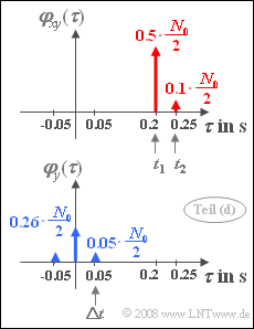
The cross-correlation function is the sum of weighted and shifted Dirac delta functions.
The cross power-spectral density is calculated as in subtask  (3).

5 Calculate the  $\rm ACF$  $\varphi_y(\tau)$  using the approximation  $\varphi_{xy}(\tau) \approx N_0/2 \cdot \delta(\tau)$.   What weights result for   $\tau = 0$   and   $\tau = \Delta t = t_2 - t_1$?

$\varphi_{y}(\tau= 0) \ = \ $ $\ \cdot 10^{-6}\ \rm W\hspace{-0.1cm}/Hz$
$\varphi_{y}(\tau= \Delta t) \ = \ $ $\ \cdot 10^{-6}\ \rm W\hspace{-0.1cm}/Hz$


Solution

(1)  The two-sided power-spectral density  ${\it \Phi}_{x}(f)$  is constantly equal  $N_0/2$  in the range  $\pm B_x$.

  • The Fourier transform is the ACF:
$$\varphi_x (\tau) = {N_0}/{2} \cdot 2 B_x \cdot {\rm sinc} (2 B_x \tau) = 0.02 \hspace {0.08cm}{\rm W} \cdot {\rm sinc} (2 B_x \tau).$$
  • Converted from   $R = 50 \hspace{0.08cm} \rm \Omega$   to   $R = 1 \hspace{0.08cm} \rm \Omega$   one obtains  $($multiplication by  $R = 50 \hspace{0.08cm} \rm \Omega)$:
$$\varphi_x (\tau) = 0.02 \hspace {0.05cm}{\rm VA} \cdot 50 \hspace {0.05cm}{\rm V/A}\cdot {\rm sinc} (2 B_x \tau)= 1 \hspace {0.05cm}{\rm V}^2 \cdot {\rm sinc} (2 B_x \tau).$$
  • The rms value is the square root of the ACF value at  $\tau = 0$:  
$$\sigma_x \hspace{0.15cm}\underline{= 1 \hspace {0.08cm}{\rm V}}.$$


(2)  For the cross correlation function  (CCF),  in the present case:

$$\varphi_{xy} (\tau) = \overline {x(t) \hspace{0.05cm}\cdot \hspace{0.05cm}y(t+\tau)} = \overline {x(t) \hspace{0.05cm}\cdot \hspace{0.05cm}\big [ \alpha_1 \cdot x(t- t_1+ \tau)\hspace{0.1cm}+\hspace{0.1cm} \alpha_2 \cdot x(t- t_2+ \tau)\big] } . $$
  • After splitting the averaging on two terms,  we get:
$$\varphi_{xy} (\tau) = \alpha_1 \cdot \overline {x(t) \hspace{0.05cm}\cdot \hspace{0.05cm} x(t- t_1+ \tau)} \hspace{0.1cm}+\hspace{0.1cm} \alpha_2 \cdot \overline {x(t) \hspace{0.05cm}\cdot \hspace{0.05cm} x(t- t_2+ \tau)} .$$
  • Using the ACF  $\varphi_x(\tau)$  can also be written:
$$\varphi_{xy} (\tau) = \alpha_1 \cdot {\varphi_{x}(\tau- t_1)} \hspace{0.1cm}+\hspace{0.1cm} \alpha_2\cdot {\varphi_{x}(\tau- t_2)} = 1 \hspace {0.08cm}{\rm V}^2 \cdot \big[ \alpha_1 \cdot {\rm sinc} (2 B_x (\tau - t_1)) + \alpha_2 \cdot {\rm sinc} (2 B_x (\tau - t_2)) \big].$$
  • The sinc–function exhibits equidistant zero crossings at all multiples of  $1/(2B_x) = 25 \hspace{0.08cm} µ \rm s$,  related to the centers at  $t_1 = 200 \hspace{0.08cm} {\rm ms}$  and  $t_2 = 250 \hspace{0.08cm} {\rm ms}$.  This results in the CCF values:
$$\varphi_{xy} (\tau = 0) \hspace{0.15cm}\underline{= 0},\hspace{0.5cm}\varphi_{xy} (\tau = t_1)= \alpha_1 \cdot \varphi_{x} (\tau = 0) \hspace{0.15cm}\underline{= 0.5\,{\rm V}^2} ,\hspace{0.5cm} \varphi_{xy} (\tau = t_2)= \alpha_2 \cdot \varphi_{x} (\tau = 0) \hspace{0.15cm}\underline{= 0.1\,{\rm V}^2} .$$


(3)  The cross power-spectral density is the Fourier transform of the CCF,  just as the power-spectral density $\rm (PSD)$  gives the Fourier transform of the ACF.  It holds:

$${\it \Phi}_{xy} (f) = \alpha_1 \cdot {\it \Phi}_{x} (f) \cdot {\rm e}^{-{\rm j}2 \pi f t_1} \hspace{0.15cm}+ \hspace{0.15cm}\alpha_2 \cdot {\it \Phi}_{x} (f) \cdot {\rm e}^{-{\rm j}2 \pi f t_2}. $$
  • Outside of the range  $|f| \le B_x$  the power-spectral density  ${\it \Phi}_{x}(f)$  – and correspondingly the cross power-spectral density  ${\it \Phi}_{xy}(f)$ – is identically zero.
  • In contrast,  inside this interval holds  ${\it \Phi}_{x}(f) = N_0/2$.  It follows in this range:
ACF and CCF with white noise
$${\it \Phi}_{xy} (f) = {N_0}/{2} \left( \alpha_1 \cdot {\rm e}^{-{\rm j}2 \pi f t_1} \hspace{0.15cm}+ \hspace{0.15cm}\alpha_2 \cdot {\rm e}^{-{\rm j}2 \pi f t_2} \right). $$
  • It is evident that  ${\it \Phi}_{xy}(f)$  unlike  ${\it \Phi}_{x}(f)$  is a complex function.  For  $f = 0$  holds:
$${\it \Phi}_{xy} (f = 0) = {N_0}/{2} \left( \alpha_1 \hspace{0.15cm}+ \hspace{0.15cm}\alpha_2 \right) = 0.3 \cdot 10^{-6}\hspace{0.05cm}{\rm W/Hz} \hspace{0.15cm}\underline{= 15 \cdot 10^{-6}\hspace{0.07cm}{\rm V^2/Hz}} . $$


(4)  Correct are  the proposed solutions 1 and 3:

  • The Fourier transform of a Dirac-shaped ACF leads to a constant PSD for all frequencies  $f$   ⇒   "true white noise".
  • This has an infinitely large power,  and for the CCF can then be written according to the above graph:
$$\varphi_{xy} (\tau) = \alpha_1 \cdot { N_0}/{2} \cdot {\rm \delta}( \tau - t_1) \hspace {0.1cm}+ \hspace {0.1cm} \alpha_2 \cdot { N_0}/{2} \cdot { \rm \delta}( \tau - t_2) .$$
  • In the frequency domain,  no difference is detectable for  $|f| \le B_x$  compared to subtask  (3)  .
  • But since  "true white noise"  is now present,  here the cross power-spectral density is not limited to this range.


(5)  For the ACF of the echoed signal,   $\varphi_{y} (\tau) = \overline {y(t) \hspace{0.05cm}\cdot \hspace{0.05cm}y(t+\tau)}$.

  • This ACF  $\varphi_{y} (\tau)$  can consequently be represented as the following sum:
$$\alpha_1^2 \cdot \overline {x(t - t_1) \cdot x(t - t_1+ \tau)} \hspace{0.03cm} + \hspace{0.03cm} \alpha_1\hspace{0.02cm}\alpha_2 \cdot \overline {x(t - t_1) \cdot x(t - t_2+ \tau)} + \hspace{0.05cm} \alpha_2\hspace{0.02cm}\alpha_1 \cdot \overline {x(t - t_2) \cdot x(t - t_1+ \tau)}\hspace{0.03cm} + \hspace{0.03cm} \alpha_2^2 \cdot \overline {x(t - t_2) \cdot x(t - t_2+ \tau)}. $$
  • For the first and the last mean:
$$\overline {x(t - t_1) \hspace{0.05cm}\cdot \hspace{0.05cm}x(t - t_1+ \tau)} = \overline {x(t - t_2) \hspace{0.05cm}\cdot \hspace{0.05cm}x(t - t_2+ \tau)} = \overline {x(t ) \hspace{0.05cm}\cdot \hspace{0.05cm}x(t + \tau)} =\varphi_x(\tau).$$
  • In contrast,  for the second and third mean values,  we obtain with  $\Delta t = t_2 - t_1= 50 \ \rm ms$:
$$\overline {x(t - t_1) \hspace{0.05cm}\cdot \hspace{0.05cm}x(t - t_2+ \tau)} = \overline {x(t ) \hspace{0.05cm}\cdot \hspace{0.05cm}x(t + t_1- t_2+ \tau)} =\varphi_x(\tau - \Delta t),$$
$$\overline {x(t - t_2) \hspace{0.05cm}\cdot \hspace{0.05cm}x(t - t_1+ \tau)} = \overline {x(t ) \hspace{0.05cm}\cdot \hspace{0.05cm}x(t + t_2- t_1+ \tau)} =\varphi_x(\tau + \Delta t).$$
  • Total,  this again results in a symmetric ACF,  as shown in the graph below:
$$\varphi_{y} (\tau) = {N_0}/{2} \cdot \left[ ( \alpha_1^2 \hspace{0.1cm} + \hspace{0.1cm} \alpha_2^2 ) \cdot {\rm \delta} (\tau) \hspace{0.1cm} + \hspace{0.1cm} \alpha_1 \cdot \alpha_2 \cdot {\rm \delta}(\tau - \delta t) \hspace{0.1cm} + \hspace{0.1cm} \alpha_1 \cdot \alpha_2 \cdot {\rm \delta}(\tau + \Delta t) \right].$$
$$\Rightarrow \hspace{0.3cm}\varphi_{y} (\tau = 0 ) \hspace{0.15cm}\underline{= 0.13 \cdot 10^{-6}\, {\rm W/Hz}},\hspace{0.3cm}\varphi_{y} (\tau = \Delta t )\hspace{0.15cm}\underline{ = 0.025 \cdot 10^{-6}\, {\rm W/Hz}}.$$