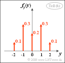
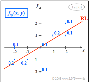
In der Grafik ist die zweidimensionale Wahrscheinlichkeitsdichtefunktion $f_{xy}(x, y)$ der zwei diskreten Zufallsgrößen $x$ und $y$ dargestellt.
The graph shows the two-dimensional probability density function $f_{xy}(x, y)$ of two discrete random variables $x$, $y$.
*Diese 2D–WDF besteht aus acht Diracpunkten, durch Kreuze markiert. Die Zahlenwerte geben die entsprechenden Wahrscheinlichkeiten an.
*This 2D–PDF consists of eight Dirac points, marked by crosses.
*Es ist zu erkennen, dass sowohl $x$ als auch $y$ alle ganzzahligen Werte zwischen den Grenzen $-2$ und $+2$ annehmen können.
*The numerical values indicate the corresponding probabilities.
*Die Varianzen der beiden Zufallsgrößen sind wie folgt gegeben: $\sigma_x^2 = 2$, $\sigma_x^2 = 1.4$.
*It can be seen that both $x$ and $y$ can take all integer values between the limits $-2$ and $+2$.
<br>
*The variances of the two random variables are given as follows: $\sigma_x^2 = 2$, $\sigma_y^2 = 1.4$.
''Hinweise:''
*Die Aufgabe gehört zum Kapitel [[Stochastische_Signaltheorie/Zweidimensionale_Zufallsgrößen|Zweidimensionale Zufallsgrößen]].
*Bezuig genommen wird auch auf das Kapitel [[Stochastische_Signaltheorie/Momente_einer_diskreten_Zufallsgröße|Momente einer diskreten Zufallsgröße]]
*Sollte die Eingabe des Zahlenwertes „0” erforderlich sein, so geben Sie bitte „0.” ein.
===Fragebogen===
Hints:
*The exercise belongs to the chapter [[Theory_of_Stochastic_Signals/Two-Dimensional_Random_Variables|Two-Dimensional Random Variables]].
*Reference is also made to the chapter [[Theory_of_Stochastic_Signals/Moments_of_a_Discrete_Random_Variable|Moments of a Discrete Random Variable]]
===Questions===
<quiz display=simple>
<quiz display=simple>
{Welche der folgenden Aussagen trefen hinsichtlich der Zufallsgröße <i>x</i> zu?
{Which of the following statements are true regarding the random variable $x$?
|type="[]"}
|type="[]"}
+ Die Wahrscheinlichkeiten für –2, –1, 0, +1 und +2 sind gleich.
+ The probabilities for $-2$, $-1$, $0$, $+1$ and $+2$ are equal.
+ Die Zufallsgröße <i>x</i> ist mittelwertfrei (<i>m<sub>x</sub></i> = 0).
+ The random variable $x$ is mean-free $(m_x = 0)$.
- Die Wahrscheinlichkeit Pr(<i>x</i> ≤ 1) ist 0.9.
- The probability ${\rm Pr}(x \le 1)=0.9$.
{Welche der folgenden Aussagen treffen hinsichtlich der Zufallsgröße <i>y</i> zu?
{Which of the following statements are true with respect to the random variable $y$?
|type="[]"}
|type="[]"}
- Die Wahrscheinlichkeiten für –2, –1, 0, +1 und +2 sind gleich.
- The probabilities for $-2$, $-1$, $0$, $+1$ and $+2$ are equal.
+ Die Zufallsgröße <i>y</i> ist mittelwertfrei (<i>m<sub>y</sub></i> = 0).
+ The random variable $y$ is mean-free $(m_y = 0)$.
+ Die Wahrscheinlichkeit Pr(<i>y</i> ≤ 1) ist 0.9.
+ The probability ${\rm Pr}(y \le 1)=0.9$.
{Berechnen Sie den Wert der zweidimensionalen VTF an der Stelle (1, 1).
{Calculate the value of the two-dimensional cumulative distribution function $\rm (CDF)$ at location $(+1, +1)$.
|type="{}"}
|type="{}"}
$F_\text{xy}(1, 1)$ = { 0.8 3% }
$F_{xy}(+1, +1) \ = \ $ { 0.8 3% }
{Berechnen Sie die Wahrscheinlichkeit, dass <i>x</i> ≤ 1 gilt, unter der Bedingung, dass gleichzeitig <i>y</i> ≤ 1 ist.
{Calculate the probability that $x \le 1$ holds, conditioned on $y \le 1$ simultaneously.
{Berechnen Sie das gemeinsame Moment der Zufallsgrößen <i>x</i> und <i>y</i>.
{Calculate the joint moment $m_{xy}$ of the random variables $x$ and $y$.
|type="{}"}
|type="{}"}
$m_\text{xy}$ = { 1.2 3% }
$m_{xy}\ = \ $ { 1.2 3% }
{Berechnen Sie den Korrelationskoeffizienten <i>ρ<sub>xy</sub></i> und geben Sie die Gleichung der Korrelationsgeraden <i>K</i>(<i>x</i>) an. Wie groß ist deren Winkel zur <i>x</i>-Achse?
{Calculate the correlation coefficient $\rho_{xy}$. Give the equation of the correlation line $K(x)$ What is its angle to the $x$–axis?
{Welche der nachfolgenden Aussagen sind zutreffend?
{Which of the following statements are true?
|type="[]"}
|type="[]"}
- Die Zufallsgrößen <i>x</i> und <i>y</i> sind statistisch unabhängig.
- The random variables $x$ and $y$ are statistically independent.
+ Man erkennt bereits aus der vorgegebenen 2D-WDF, dass <i>x</i> und <i>y</i> statistisch voneinander abhängen.
+ It can already be seen from the given 2D–PDF that $x$ and $y$ are statistically dependent on each other.
+ Aus dem berechneten Korrelationskoeffizienten <i>ρ<sub>xy</sub></i> kann man auf die statistische Abhängigkeit zwischen <i>x</i> und <i>y</i> schließen.
+ From the calculated correlation coefficient $\rho_{xy}$ one can conclude the statistical dependence between $x$ and $y$ .
Line 63:
Line 70:
</quiz>
</quiz>
===Musterlösung===
===Solution===
{{ML-Kopf}}
{{ML-Kopf}}
:<b>1.</b> Die Randwahrscheinlichkeitsdichtefunktion <i>f<sub>x</sub></i>(<i>x</i>) erhält man aus der 2D–WDF <i>f<sub>xy</sub></i>(<i>x, y</i>) durch Integration über <i>y</i>. Für alle möglichen Werte <i>x</i> ∈ {–2, –1, 0, 1, 2} sind die Wahrscheinlichkeiten gleich 0.2, und es gilt Pr(<i>x</i> ≤ 1) = 0.8. Der Mittelwert ist <i>m<sub>x</sub></i> = 0. Richtig sind somit <u>die beiden ersten Antworten</u>.
'''(1)''' Correct are the <u>first two answers</u>:
[[File:P_ID258__Sto_Z_4_3_b.png|right|]]
*The marginal probability density function $f_{x}(x)$ is obtained from the 2D–PDF $f_{xy}(x, y)$ by integration over $y$.
*For all possible values $ x \in \{-2, -1, \ 0, +1, +2\}$ the probabilities are equal $0.2$.
*It holds ${\rm Pr}(x \le 1)= 0.8$. The mean is $m_x = 0$.
:<b>2.</b> Durch Integration über <i>x</i> erhält man die rechts skizzierte WDF. Aufgrund der Symmetrie ergibt sich der Mittelwert <i>m<sub>y</sub></i> = 0. Die gesuchte Wahrscheinlichkeit Pr(<i>y</i> ≤ 1) ist 0.9. Richtig sind also <u>die Lösungsvorschläge 2 und 3</u>.<br>
*As can be seen from the 2D–PDF on the information page, this probability is ${\rm Pr}\big [(x \le 1)\cap(y\le 1)\big ]\hspace{0.15cm}\underline{=0.8}$.
:Mit den Ergebnissen aus (2) und (3) folgt daraus Pr(<i>x</i> ≤ 1 | <i>y</i> ≤ 1) = 0.8/0.9 = 8/9 <u>= 0.889</u>.
:<b>5.</b> Entsprechend der Definition gilt für das gemeinsame Moment:
:Hier ist berücksichtigt, dass wegen <i>m<sub>x</sub></i> = <i>m<sub>y</sub></i> = 0 die Kovarianz <i>μ<sub>xy</sub></i> gleich dem Moment <i>m<sub>xy</sub></i> ist.
:Die Gleichung der Korrelationsgeraden lautet:
[[File:EN_Sto_Z_4_3_f.png|right|frame|2D–PDF and regression line $\rm (RL)$]]
*This takes into account that because $m_x = m_y = 0$ the covariance $\mu_{xy}$ is equal to the moment $m_{xy}$ .
*The equation of the correlation line is:
:$$y=\frac{\sigma_y}{\sigma_x}\cdot \rho_{xy}\cdot x = \frac{\mu_{xy}}{\sigma_x^{\rm 2}}\cdot x = \rm 0.6\cdot \it x.$$
:$$y=\frac{\sigma_y}{\sigma_x}\cdot \rho_{xy}\cdot x = \frac{\mu_{xy}}{\sigma_x^{\rm 2}}\cdot x = \rm 0.6\cdot \it x.$$
:Im Bild ist die Gerade <i>y</i> = <i>K</i>(<i>x</i>) eingezeichnet. Der Winkel zwischen Korrelationsgerade und <i>x</i>-Achse beträgt <i>θ</i><sub><i>y</i>→<i>x</i></sub> = arctan(0.6) <u>≈ 31°</u>.
*See sketch on the right. The angle between the regression line $\rm (RL)$ and the $x$-axis is
:<b>7.</b> Bei statistischer Unabhängigkeit müsste <i>f<sub>xy</sub></i>(<i>x</i>, <i>y</i>) = <i>f<sub>x</sub></i>(<i>x</i>) · <i>f<sub>y</sub></i>(<i>y</i>) gelten, was hier nicht erfüllt ist. Aus der Korreliertheit (folgt aus <i>ρ<sub>xy</sub></i> = 0.6) kann direkt auf die statistische Abhängigkeit geschlossen werden, denn Korrelation bedeutet eine Sonderform (nämlich linear) der statistischen Abhängigkeit. Richtig sind die <u>Lösungsvorschläge 2 und 3</u>.
'''(7)''' The correct solutions are <u>solutions 2 and 3</u>:
*If statistically independent, $f_{xy}(x, y) = f_{x}(x) \cdot f_{y}(y)$ should hold, which is not done here.
*From correlatedness $($follows from $\rho_{xy} \ne 0)$ it is possible to directly infer statistical dependence,
*because correlation means a special form of statistical dependence, namely linear statistical dependence.
{{ML-Fuß}}
{{ML-Fuß}}
Line 106:
Line 133:
[[Category:Aufgaben zu Stochastische Signaltheorie|^4.1 Zweidimensionale Zufallsgrößen^]]
[[Category:Theory of Stochastic Signals: Exercises|^4.1 Two-Dimensional Random Variables^]]
As can be seen from the 2D–PDF on the information page, this probability is ${\rm Pr}\big [(x \le 1)\cap(y\le 1)\big ]\hspace{0.15cm}\underline{=0.8}$.
(4) For this, Bayes' theorem can also be used to write:
With the results from (2) and (3) it follows $ \rm Pr(\it x \le \rm 1)\hspace{0.05cm} | \hspace{0.05cm} \it y \le \rm 1) = 0.8/0.9 = 8/9 \hspace{0.15cm}\underline{=0.889}$.
(5) According to the definition, the common moment is: