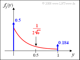
Dieses Signal wird an den Eingang einer Nichtlinearität mit der Kennlinie (siehe unteres Bild) angelegt:
*This signal is applied to the input of a nonlinearity with the characteristic curve (see lower figure):
$$y=\left\{\begin{array}{*{4}{c}}0 &\rm f\ddot{u}r\hspace{0.2cm} \it x <\rm 0, \\\rm2\it x & \rm f\ddot{u}r\hspace{0.2cm} \rm 0\le \it x\le \rm 0.5, \\1 & \rm f\ddot{u}r\hspace{0.2cm}\it x > \rm 0.5\\\end{array}\right.$$
:$$y=\left\{\begin{array}{*{4}{c}}0 &\rm for\hspace{0.2cm} \it x <\rm 0, \\\rm2\it x & \rm for\hspace{0.2cm} \rm 0\le \it x\le \rm 0.5, \\1 & \rm for\hspace{0.2cm}\it x > \rm 0.5\\\end{array}\right.$$
Das Ausgangssignal wird mit $y(t)$ bezeichnet.
*The characteristic sketched below limits the variable $x(t)$ at the input asymmetrically and amplifies it in the linear range.<br><br>
Diese unten skizzierte Kennlinie begrenzt die Größe $x(t)$ am Eingang asymmetrisch und verstärkt sie im linearen Bereich.<br><br>
''Hinweise:''
*Die Aufgabe gehört zum Kapitel [[Stochastische_Signaltheorie/Exponentialverteilte_Zufallsgrößen|Exponentialverteilte Zufallsgröße]].
*Sollte die Eingabe des Zahlenwertes „0” erforderlich sein, so geben Sie bitte „0.” ein.
*Gegeben ist das folgende bestimmte Integral:
Hints:
*The exercise belongs to the chapter [[Theory_of_Stochastic_Signals/Exponentially_Distributed_Random_Variables|Exponentially Distributed Random Variable]].
* Use the HTML5/JavaScript– applet [[Applets:PDF,_CDF_and_Moments_of_Special_Distributions|PDF, CDF and Moments of Special Distributions]] to check your results.
{Berechnen Sie den Funktionswert $A= f_x(0)$ der WDF an der Stelle $x = 0$.
{Calculate the function value $A= f_x(0)$ of the PDF at the location $x = 0$.
|type="{}"}
|type="{}"}
$A \ =$ { 1 3% }
$A \ = \ $ { 1 3% }
{Berechnen Sie die Momente $m_k$ der Zufallsgröße $x$. Begründen Sie, dass alle Momente mit ungeradem Index null sind. Wie groß ist die Streuung?
{Calculate the moments $m_k$ of the random variable $x$. Reason that all moments with odd index are zero. How big is the standard deviation?
|type="{}"}
|type="{}"}
$\sigma_x \ =$ { 0.707 3% }
$\sigma_x \ = \ $ { 0.707 3% }
{Welcher Wert ergibt sich für die Kurtosis der Zufallsgröße $x$?
{What is the value of the kurtosis of the random variable $x$?
|type="{}"}
|type="{}"}
$K_x \ =$ { 6 3% }
$K_x \ = \ $ { 6 3% }
{Wie groß ist die Wahrscheinlichkeit, dass $x$ den Wert $0.5$ überschreitet?
{What is the probability that $x$ exceeds $0.5$ ?
|type="{}"}
|type="{}"}
${\rm Pr}(x > 0.5) \ =$ { 0.184 3% }
${\rm Pr}(x > 0.5) \ = \ $ { 18.4 3% } $\ \%$
{Welche der folgenden Aussagen sind bezüglich der WDF $f_y(y)$ zutreffend?
{Which of the following statements are true regarding the PDF $f_y(y)$ ?
|type="[]"}
|type="[]"}
+ Die WDF beinhaltet eine Diracfunktion bei $y = 0$.
+ The PDF contains a Dirac delta function at $y = 0$.
- Die WDF beinhaltet eine Diracfunktion bei $y = 0.5$.
- The PDF contains a Dirac delta function at $y = 0.5$.
+ Die WDF beinhaltet eine Diracfunktion bei $y = 1$.
+ The PDF contains a Dirac delta function at $y = 1$.
{Wie lautet der kontinuierliche Anteil der WDF $f_y(y)$? Welcher Wert ergibt sich für $y = 0.5$?
{What is the continuous part of the PDF $f_y(y)$? What value results for $y = 0.5$ ?
|type="{}"}
|type="{}"}
$f_y(y = 0.5) \ =$ { 0.304 3% }
$f_y(y = 0.5) \ = \ $ { 0.304 3% }
{Wie groß ist der Mittelwert der begrenzten und verstärkten Zufallsgröße $y$?
{What is the mean of the bounded and amplified random variable $y$?
|type="{}"}
|type="{}"}
$m_y \ =$ { 0.316 3% }
$m_y \ = \ $ { 0.316 3% }
</quiz>
</quiz>
===Musterlösung===
===Solution===
{{ML-Kopf}}
{{ML-Kopf}}
'''(1)''' Die Fläche unter der Wahrscheinlichkeitsdichtefunktion ergibt
'''(1)''' The area under the probability density function yields
Da diese Fläche definitionsgemäß gleich $F = 1$ sein muss, gilt $\underline{A = 1}$.
'''(2)''' Alle Momente mit ungeradem Index $k$ sind aufgrund der symmetrischen WDF gleich Null. Bei geradem $k$ kann der linke Teil der WDF in den rechten gespiegelt werden und man erhält:
'''(4)''' Using the result from '''(1)''' we get:
'''(6)''' Der Signalbereich $0 \le x \le 0.5$ wird am Ausgang auf den Bereich $0 \le y \le 1$ linear abgebildet. Die Ableitung der Kennlinie ist hier konstant gleich $2$ (Verstärkung). Daraus erhält man:
*For $y= 0.5$ accordingly, the continuous PDF component is