Difference between revisions of "Aufgaben:Exercise 4.2: Triangle Area again"
m (Guenter verschob die Seite 4.2 Wieder Dreieckgebiet nach Aufgabe 4.2: Wieder Dreieckgebiet) |
|||
| (15 intermediate revisions by 5 users not shown) | |||
| Line 1: | Line 1: | ||
| − | {{quiz-Header|Buchseite= | + | {{quiz-Header|Buchseite=Theory_of_Stochastic_Signals/Two-Dimensional_Random_Variables |
}} | }} | ||
| − | [[File:P_ID226__Sto_A_4_2.png|right| | + | [[File:P_ID226__Sto_A_4_2.png|right|frame|Triangular 2D area and the two marginal probability densities]] |
| − | + | We consider the same random variable $(x, \ y)$ as in [[Aufgaben:Exercise_4.1:_Triangular_(x,_y)_Area|Exercise 4.1]]: | |
| − | *In | + | *In a domain defined by vertices $(0,\ 1)$, $(4,\ 3)$, and $(4,\ 5)$ let the 2D–PDF $f_{xy} (x, y) = 0.25$. |
| + | *There are no values outside this definition area $D$ marked in red in the graph. | ||
| − | + | Furthermore, the two marginal probability densities with respect to the quantities $x$ and $y$ are drawn in the graph, which have already been determined in Exercise 4.1. | |
| − | |||
| − | |||
| − | + | From this, the equations of chapter [[Theory_of_Stochastic_Signals/Expected_Values_and_Moments|Expected Values and Moments]] can be used to determine the characteristics of the two random variables: | |
| − | $$ | + | :$$m_x=8/3 ,\hspace{0.5cm} \sigma_x=\sqrt{8/9},$$ |
| + | :$$ m_y= 3,\hspace{0.95cm} \sigma_y = \sqrt{\rm 2/3}.$$ | ||
| + | Due to the fact that the definition domain $D$ is bounded by two straight lines $y_1(x)$ and $y_2(x)$ , the first order joint moment can be calculated here as follows. | ||
| + | :$$m_{xy}={\rm E}\big[x\cdot y\big]=\int_{x_{1}}^{x_{2}}x\cdot \int_{y_{1}(x)}^{y_{2}(x)}y \cdot f_{xy}(x,y) \, \,{\rm d}y\, {\rm d}x.$$ | ||
| − | |||
| − | |||
| − | |||
| − | |||
| − | === | + | |
| + | |||
| + | |||
| + | |||
| + | Hints: | ||
| + | *The Exercise belongs to the chapter [[Theory_of_Stochastic_Signals/Two-Dimensional_Random_Variables|Two-Dimensional Random Variables]]. | ||
| + | *Reference is also made to the chapter [[Theory_of_Stochastic_Signals/Expected_Values_and_Moments|Expected Values and Moments]]. | ||
| + | |||
| + | |||
| + | |||
| + | |||
| + | ===Questions=== | ||
<quiz display=simple> | <quiz display=simple> | ||
| − | { | + | {What are the limit lines of the inner integral for the $m_{xy}$ calculation? |
| − | |type=" | + | |type="()"} |
- $y_1(x) = x+1, $ $y_2(x) = 2x+1.$ | - $y_1(x) = x+1, $ $y_2(x) = 2x+1.$ | ||
+ $y_1(x) = x/2+1, $ $y_2(x) = x+1.$ | + $y_1(x) = x/2+1, $ $y_2(x) = x+1.$ | ||
| Line 33: | Line 42: | ||
| − | { | + | {Calculate the joint moment $m_{xy}$ according to the double integral on the statement page. <i>Note</i>: Set $x_1 = 0$ and $x_2 = 4$. |
|type="{}"} | |type="{}"} | ||
| − | $m_{xy} \ =$ | + | $m_{xy} \ = \ $ { 8.667 3% } |
| − | { | + | {What is the covariance $\mu_{xy}$ ? |
|type="{}"} | |type="{}"} | ||
| − | $\mu_{xy}\ =$ { 0.667 3% } | + | $\mu_{xy}\ = \ $ { 0.667 3% } |
| − | { | + | {What is the correlation coefficient $\rho_{xy}$? |
|type="{}"} | |type="{}"} | ||
| − | $\rho_{xy}\ =$ { 0.866 3% } | + | $\rho_{xy}\ = \ $ { 0.866 3% } |
| − | { | + | {What is the equation of the regression line $y = K(x)$? At what point $y_0$ does the straight line intersect the $y$–axis? <br>Show that the correlation line also passes through the point $(m_x, m_y)$. |
|type="{}"} | |type="{}"} | ||
| − | $y_0\ =$ { 1 3% } | + | $y_0\ = \ $ { 1 3% } |
| Line 56: | Line 65: | ||
</quiz> | </quiz> | ||
| − | === | + | ===Solution=== |
{{ML-Kopf}} | {{ML-Kopf}} | ||
| − | '''(1)''' | + | '''(1)''' Correct is the <u>middle proposition</u>: |
| − | * | + | *Both $y_1(x)$ and $y_2(x)$ intersect the $y$-axis at $y= 1$. |
| − | * | + | *The lower boundary line has slope $0.5$, the upper has slope $1$. |
| − | |||
| − | |||
| − | + | '''(2)''' According to the clues we get: | |
| − | :$$m_{xy}= | + | : $$m_{xy}=\int_{\rm 0}^{\rm 4} x \cdot \int_{\it x/\rm 2 +\rm 1}^{\it x+\rm 1} {1}/{4}\cdot y \, \,{\rm d}y\,\, {\rm d}x = {1}/{8}\cdot \int_{\rm 0}^{\rm 4} x\cdot \big[( x+ 1)^{\rm 2}- ({ x}/{2}+1)^{\rm 2} \big] \,\, {\rm d}x. $$ |
| − | '''(3)''' | + | *This leads to the integral or final result: |
| + | :$$m_{xy}={1}/{8}\int_{\rm 0}^{\rm 4}(\frac{3}{4}\cdot x^{3}{\rm +} x^2\,{\rm d}x = \rm \frac{1}{8} \cdot (\frac{3}{16}\cdot 4^4+\rm \frac{4^3}{3})=\frac{26}{3}\hspace{0.15cm}\underline{ \approx 8.667}.$$ | ||
| + | |||
| + | '''(3)''' Since both random variables each have a nonzero mean, it follows for the covariance: | ||
| + | [[File:EN_Sto_Z_4_2d.png|right|frame|Regression line]] | ||
:$$\it \mu_{xy}=\it m_{xy}-m_{x}\cdot m_{y}=\frac{\rm 26}{\rm 3}-\frac{\rm 8}{\rm 3}\cdot\rm 3={2}/{3} \hspace{0.15cm}\underline{=0.667}.$$ | :$$\it \mu_{xy}=\it m_{xy}-m_{x}\cdot m_{y}=\frac{\rm 26}{\rm 3}-\frac{\rm 8}{\rm 3}\cdot\rm 3={2}/{3} \hspace{0.15cm}\underline{=0.667}.$$ | ||
| − | '''(4)''' | + | '''(4)''' With the given standard deviations we obtain: |
:$$\rho_{xy}=\frac{\mu_{xy}}{\sigma_{x}\cdot\sigma_{y}}=\frac{{\rm 2}/{\rm 3}}{\sqrt{{\rm 8}/{\rm 9}}\cdot\sqrt{{\rm 2}/{\rm 3}}}=\sqrt{0.75}\hspace{0.15cm}\underline{=\rm 0.866}.$$ | :$$\rho_{xy}=\frac{\mu_{xy}}{\sigma_{x}\cdot\sigma_{y}}=\frac{{\rm 2}/{\rm 3}}{\sqrt{{\rm 8}/{\rm 9}}\cdot\sqrt{{\rm 2}/{\rm 3}}}=\sqrt{0.75}\hspace{0.15cm}\underline{=\rm 0.866}.$$ | ||
| − | |||
| − | '''(5)''' | + | '''(5)''' For the regression line ("RL" in the graph), in general: |
:$$ y-m_{y}=\rho_{xy}\cdot\frac{\sigma_{y}}{\sigma_ {x}}\cdot(x-m_{x}).$$ | :$$ y-m_{y}=\rho_{xy}\cdot\frac{\sigma_{y}}{\sigma_ {x}}\cdot(x-m_{x}).$$ | ||
| − | + | *Using the numerical values calculated above, we obtain | |
| − | + | :$$y={\rm 3}/{\rm 4}\cdot x +\rm 1.$$ | |
| − | $$y={\rm 3}/{\rm 4}\cdot | + | *The correlation line intersects the $y$-axis at $\underline{y=1}$ and also passes through the point $(4, 4)$. |
| − | + | *Any other result would be impossible to interpret considering the definition area: | |
| − | + | ::If one sets $m_x = 8/3$, one obtains $y = m_y = 3$. | |
| − | + | *This means: The calculated correlation line actually passes through the point $(m_x, m_y)$, as the theory says. | |
| − | * | ||
{{ML-Fuß}} | {{ML-Fuß}} | ||
| − | [[Category: | + | [[Category:Theory of Stochastic Signals: Exercises|^4.1 Two-Dimensional Random Variables^]] |
Latest revision as of 17:43, 13 March 2023
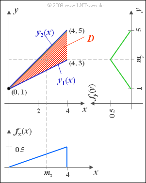
We consider the same random variable $(x, \ y)$ as in Exercise 4.1:
- In a domain defined by vertices $(0,\ 1)$, $(4,\ 3)$, and $(4,\ 5)$ let the 2D–PDF $f_{xy} (x, y) = 0.25$.
- There are no values outside this definition area $D$ marked in red in the graph.
Furthermore, the two marginal probability densities with respect to the quantities $x$ and $y$ are drawn in the graph, which have already been determined in Exercise 4.1.
From this, the equations of chapter Expected Values and Moments can be used to determine the characteristics of the two random variables:
- $$m_x=8/3 ,\hspace{0.5cm} \sigma_x=\sqrt{8/9},$$
- $$ m_y= 3,\hspace{0.95cm} \sigma_y = \sqrt{\rm 2/3}.$$
Due to the fact that the definition domain $D$ is bounded by two straight lines $y_1(x)$ and $y_2(x)$ , the first order joint moment can be calculated here as follows.
- $$m_{xy}={\rm E}\big[x\cdot y\big]=\int_{x_{1}}^{x_{2}}x\cdot \int_{y_{1}(x)}^{y_{2}(x)}y \cdot f_{xy}(x,y) \, \,{\rm d}y\, {\rm d}x.$$
Hints:
- The Exercise belongs to the chapter Two-Dimensional Random Variables.
- Reference is also made to the chapter Expected Values and Moments.
Questions
Solution
- Both $y_1(x)$ and $y_2(x)$ intersect the $y$-axis at $y= 1$.
- The lower boundary line has slope $0.5$, the upper has slope $1$.
(2) According to the clues we get:
- $$m_{xy}=\int_{\rm 0}^{\rm 4} x \cdot \int_{\it x/\rm 2 +\rm 1}^{\it x+\rm 1} {1}/{4}\cdot y \, \,{\rm d}y\,\, {\rm d}x = {1}/{8}\cdot \int_{\rm 0}^{\rm 4} x\cdot \big[( x+ 1)^{\rm 2}- ({ x}/{2}+1)^{\rm 2} \big] \,\, {\rm d}x. $$
- This leads to the integral or final result:
- $$m_{xy}={1}/{8}\int_{\rm 0}^{\rm 4}(\frac{3}{4}\cdot x^{3}{\rm +} x^2\,{\rm d}x = \rm \frac{1}{8} \cdot (\frac{3}{16}\cdot 4^4+\rm \frac{4^3}{3})=\frac{26}{3}\hspace{0.15cm}\underline{ \approx 8.667}.$$
(3) Since both random variables each have a nonzero mean, it follows for the covariance:
- $$\it \mu_{xy}=\it m_{xy}-m_{x}\cdot m_{y}=\frac{\rm 26}{\rm 3}-\frac{\rm 8}{\rm 3}\cdot\rm 3={2}/{3} \hspace{0.15cm}\underline{=0.667}.$$
(4) With the given standard deviations we obtain:
- $$\rho_{xy}=\frac{\mu_{xy}}{\sigma_{x}\cdot\sigma_{y}}=\frac{{\rm 2}/{\rm 3}}{\sqrt{{\rm 8}/{\rm 9}}\cdot\sqrt{{\rm 2}/{\rm 3}}}=\sqrt{0.75}\hspace{0.15cm}\underline{=\rm 0.866}.$$
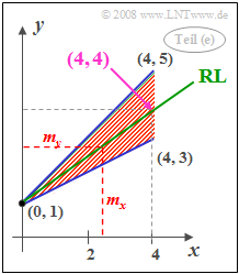
(5) For the regression line ("RL" in the graph), in general:
- $$ y-m_{y}=\rho_{xy}\cdot\frac{\sigma_{y}}{\sigma_ {x}}\cdot(x-m_{x}).$$
- Using the numerical values calculated above, we obtain
- $$y={\rm 3}/{\rm 4}\cdot x +\rm 1.$$
- The correlation line intersects the $y$-axis at $\underline{y=1}$ and also passes through the point $(4, 4)$.
- Any other result would be impossible to interpret considering the definition area:
- If one sets $m_x = 8/3$, one obtains $y = m_y = 3$.
- This means: The calculated correlation line actually passes through the point $(m_x, m_y)$, as the theory says.

