Aufgaben:Exercise 3.8: Amplification and Limitation: Difference between revisions

From LNTwww
No edit summary
Fix interlanguage link: resolve redirect chain
 
(18 intermediate revisions by 5 users not shown)
Line 1: Line 1:


{{quiz-Header|Buchseite=Stochastische Signaltheorie/Exponentialverteilte Zufallsgrößen
{{quiz-Header|Buchseite=Theory_of_Stochastic_Signals/Exponentially_Distributed_Random_Variables
}}
}}


[[File:P_ID130__Sto_A_3_8.png|right|frame|Verstärkung und Begrenzung der Zufallsgröße $x$]]
[[File:P_ID130__Sto_A_3_8.png|right|frame|Amplification and limitation<br>of the random variable&nbsp; $x$]]
Wir betrachten ein Zufallssignal $x(t)$ mit symmetrischer Wahrscheinlichkeitsdichtefunktion:
We consider a random signal&nbsp; $x(t)$&nbsp; with symmetric probability density function&nbsp; $\rm (PDF)$:
:$$f_x(x)=A\cdot \rm e^{\rm -2 \hspace{0.05cm}\cdot \hspace{0.05cm}|\it x|}.$$


*Dieses Signal wird an den Eingang einer Nichtlinearit&auml;t mit der Kennlinie (siehe unteres Bild) angelegt:
*This signal is applied to the input of a nonlinearity with the characteristic curve&nbsp; (see lower figure):
:$$y=\left\{\begin{array}{*{4}{c}}0  &\rm f\ddot{u}r\hspace{0.2cm} \it x <\rm 0, \\\rm2\it x  & \rm f\ddot{u}r\hspace{0.2cm} \rm 0\le \it x\le \rm 0.5,  \\1 & \rm f\ddot{u}r\hspace{0.2cm}\it x > \rm 0.5\\\end{array}\right.$$
:$$y=\left\{\begin{array}{*{4}{c}}0  &\rm for\hspace{0.2cm} \it x <\rm 0, \\\rm2\it x  & \rm for\hspace{0.2cm} \rm 0\le \it x\le \rm 0.5,  \\1 & \rm for\hspace{0.2cm}\it x > \rm 0.5\\\end{array}\right.$$


*Das Ausgangssignal wird mit $y(t)$ bezeichnet.  
*The characteristic sketched below limits the variable&nbsp; $x(t)$&nbsp; at the input asymmetrically and amplifies it in the linear range.<br><br>


*Die unten skizzierte Kennlinie begrenzt die Gr&ouml;&szlig;e $x(t)$ am Eingang asymmetrisch und  verst&auml;rkt sie im linearen Bereich.<br><br>


Line 18: Line 17:


''Hinweise:''
 
*Die Aufgabe gehört zum  Kapitel [[Stochastische_Signaltheorie/Exponentialverteilte_Zufallsgrößen|Exponentialverteilte Zufallsgröße]].
Hints:
*The exercise belongs to the chapter&nbsp; [[Theory_of_Stochastic_Signals/Exponentially_Distributed_Random_Variables|Exponentially Distributed Random Variable]].
*Gegeben ist das folgende bestimmte Integral:
* Use the HTML5/JavaScript&ndash; applet&nbsp; [[Applets:PDF,_CDF_and_Moments_of_Special_Distributions|PDF, CDF and Moments of Special Distributions]]&nbsp; to check your results.
*Given the following definite integral:
:$$\int_{0}^{\infty}\it x^n\cdot\rm e^{-\it a \hspace{0.03cm}\cdot \hspace{0.03cm}x}\, d{\it x} =\frac{\it n{\rm !}}{\it a^{n}}.$$


===Fragebogen===
===Questions===


<quiz display=simple>
{Berechnen Sie den Funktionswert $A= f_x(0)$ der WDF an der Stelle $x = 0$.
{Calculate the function value&nbsp; $A= f_x(0)$&nbsp; of the PDF at the location&nbsp; $x = 0$.
|type="{}"}
|type="{}"}
$A \ = \ $ { 1 3% }
$A \ = \ $ { 1 3% }


{Berechnen Sie die Momente $m_k$ der Zufallsgr&ouml;&szlig;e $x$. Begr&uuml;nden Sie, dass alle Momente mit ungeradem Index Null sind. <br>Wie groß ist die Streuung?
{Calculate the moments&nbsp; $m_k$&nbsp; of the random variable&nbsp; $x$.&nbsp; Reason that all moments with odd index are zero.&nbsp; How big is the standard deviation?
|type="{}"}
|type="{}"}
$\sigma_x \ = \ $ { 0.707 3% }


{Welcher Wert ergibt sich f&uuml;r die Kurtosis der Zufallsgr&ouml;&szlig;e $x$?
{What is the value of the kurtosis of the random variable&nbsp; $x$?
|type="{}"}
|type="{}"}
$K_x \ = \ $ { 6 3% }


{Wie gro&szlig; ist die Wahrscheinlichkeit, dass $x$ den Wert $0.5$ &uuml;berschreitet?
{What is the probability that&nbsp; $x$&nbsp; exceeds&nbsp; $0.5$&nbsp;?
|type="{}"}
|type="{}"}
${\rm Pr}(x > 0.5) \ = \ $ { 0.184 3% }
${\rm Pr}(x > 0.5) \ = \ $ { 18.4 3% } $\ \%$


{Welche der folgenden Aussagen sind bez&uuml;glich der WDF $f_y(y)$ zutreffend?
{Which of the following statements are true regarding the PDF&nbsp; $f_y(y)$&nbsp;?
|type="[]"}
|type="[]"}
+ Die WDF beinhaltet eine Diracfunktion bei $y = 0$.
+ The PDF contains a Dirac delta function at&nbsp; $y = 0$.
- Die WDF beinhaltet eine Diracfunktion bei $y = 0.5$.
- The PDF contains a Dirac delta function at&nbsp; $y = 0.5$.
+ Die WDF beinhaltet eine Diracfunktion bei $y = 1$.
+ The PDF contains a Dirac delta function at&nbsp; $y = 1$.


{Wie lautet der kontinuierliche Anteil der WDF $f_y(y)$? Welcher Wert ergibt sich f&uuml;r $y = 0.5$?
{What is the continuous part of the PDF&nbsp; $f_y(y)$?&nbsp; What value results for&nbsp; $y = 0.5$&nbsp;?
|type="{}"}
|type="{}"}
$f_y(y = 0.5) \ = \ $ { 0.304 3% }


{Wie groß ist der Mittelwert der begrenzten und verst&auml;rkten Zufallsgr&ouml;&szlig;e $y$?
{What is the mean of the bounded and amplified random variable&nbsp; $y$?
|type="{}"}
|type="{}"}
$m_y \ = \ $ { 0.316 3% }


</quiz>
</quiz>


===Musterlösung===
===Solution===
{{ML-Kopf}}
{{ML-Kopf}}
'''(1)'''&nbsp; Die Fl&auml;che unter der Wahrscheinlichkeitsdichtefunktion ergibt
'''(1)'''&nbsp; The area under the probability density function yields
:$$\it F=\rm 2\cdot \it A\int_{\rm 0}^{\infty}\hspace{-0.15cm}\rm e^{\rm -2\it x}\, \rm d \it x=\frac{\rm 2\cdot \it A}{\rm -2}\cdot \rm e^{\rm -2\it x}\Big|_{\rm 0}^{\infty}=\it A.$$


Da diese Fl&auml;che definitionsgem&auml;&szlig; gleich $F = 1$ sein muss, gilt $\underline{A = 1}$.
*Since this area must be equal by definition&nbsp; $F = 1$ &nbsp; &rArr; &nbsp; $\underline{A = 1}$.


'''(2)'''&nbsp; Alle Momente mit ungeradem Index $k$ sind aufgrund der symmetrischen WDF gleich Null. Bei geradem $k$ kann der linke Teil der WDF in den rechten gespiegelt werden und man erh&auml;lt:
'''(2)'''&nbsp; All moments with odd index&nbsp; $k$&nbsp; are equal to zero due to the symmetrical PDF.  
*For even&nbsp; $k$&nbsp; the left part of the PDF can be mirrored into the right one and we get:
:$$\it m_k=\rm 2 \cdot \int_{\rm 0}^{\infty}\hspace{-0.15cm}\it x^{k}\cdot \rm e^{-\rm 2\it x}\,\rm d \it x=\frac{\rm 2\cdot\rm\Gamma(\it k{\rm +}\rm 1)}{\rm 2^{\it k{\rm +}\rm 1}}=\frac{\it k{\rm !}}{\rm 2^{\it k}}.$$


Daraus folgt mit $k = 2$ unter Berücksichtigung des Mittelwertes $m_1 = 0$:
*From this it follows with&nbsp; $k = 2$&nbsp; considering the mean&nbsp; $m_1 = 0$:
$$m_{\rm 2}=\frac{\rm 2!}{\rm 2^2}={\rm 0.5\hspace{0.5cm}bzw.\hspace{0,5cm} }\sigma_x=\sqrt{ m_{\rm 2}}\hspace{0.15cm}\underline{=\rm 0.707}.$$
:$$m_{\rm 2}=\frac{\rm 2!}{\rm 2^2}={\rm 0.5\hspace{0.5cm}bzw.\hspace{0.5cm} }\sigma_x=\sqrt{ m_{\rm 2}}\hspace{0.15cm}\underline{=\rm 0.707}.$$


'''(3)'''&nbsp; Das Zentralmoment vierter Ordnung ist $\mu_4 = m_4 = 4!/2^4 = 1.5$. Daraus folgt für die Kurtosis:
[[File:P_ID131__Sto_A_3_8_e.png|right|frame|PDF after amplification and boundary]]
[[File:P_ID131__Sto_A_3_8_e.png|right|frame|WDF nach Verstärkung und Begrenzung]]
'''(3)'''&nbsp; The fourth-order central moment is&nbsp; $\mu_4 = m_4 = 4!/2^4 = 1.5$.  
*From this follows for the kurtosis:
:$$K_{x}=\frac{ \mu_{\rm 4}}{ \sigma_{\it x}^{4}}=\frac{1.5}{0.25}\hspace{0.15cm}\underline{=\rm 6}.$$


'''(4)'''&nbsp; Mit dem Ergebnis aus '''(1)''' erh&auml;lt man:  
'''(4)'''&nbsp; Using the result from&nbsp; '''(1)'''&nbsp; we get:  
:$${\rm Pr}( x> 0.5)=\int_{0.5}^{\infty}{\rm e}^{- 2 x}\,{\rm d}t x=\frac{\rm 1}{\rm 2\rm e}\hspace{0.15cm}\underline{=\rm 0.184}.$$
:$${\rm Pr}( x> 0.5)=\int_{0.5}^{\infty}{\rm e}^{- 2 x}\,{\rm d}x=\frac{\rm 1}{\rm 2\rm e}\hspace{0.15cm}\underline{=\rm 18.4\%}.$$
 
 
'''(5)'''&nbsp; Correct are the&nbsp; <u>solutions 1 and 3</u>:
*The PDF&nbsp; $f_y(y)$&nbsp; involves a Dirac delta function at the point&nbsp; $y= 0$&nbsp; with weight&nbsp; ${\rm Pr}(x < 0) = 0.5$.
*In addition,&nbsp; another Dirac delta function at&nbsp; $y= 1$&nbsp; with weight&nbsp; ${\rm Pr}(x > 0.5) = 0.184$.


'''(5)'''&nbsp; Richtig sind  die <u>Lösungsvorschläge 1 und 3</u>:
'''(6)'''&nbsp; The signal range&nbsp; $0 \le x \le 0.5$&nbsp; is linearly mapped to the range&nbsp; $0 \le y \le 1$&nbsp; at the output.  
*Die WDF $f_y(y)$ beinhaltet eine Diracfunktion an der Stelle $y= 0$ mit dem Gewicht ${\rm Pr}(x < 0) = 0.5$.
*The derivative of the characteristic curve is constantly equal to $2$&nbsp; (amplification). From this one obtains:
*Zudem eine weitere Diracfunktion bei $y= 1$ mit dem Gewicht ${\rm Pr}(x > 0.5) = 0.184$.
<br clear=all>
'''(6)'''&nbsp; Der Signalbereich $0 \le x \le 0.5$ wird am Ausgang auf den Bereich $0 \le y \le 1$ linear abgebildet. Die Ableitung der Kennlinie ist hier konstant gleich $2$ (Verst&auml;rkung). Daraus erh&auml;lt man:
:$$f_y(y)=\frac{f_x(x)}{|g'(x)|}\Bigg|_{x=h(y)}=\frac{\rm e^{-\rm 2\it x}}{\rm 2}\Bigg|_{\it x={\it y}/{\rm 2}}=0.5 \cdot {\rm e^{\it -y}} .$$


Bei $y= 0.5$ beträgt dementsprechend der kontinuierliche WDF-Anteil $f_y(y = 0.5)\hspace{0.15cm}\underline{\approx 0.304}$.
*For&nbsp; $y= 0.5$&nbsp; accordingly,&nbsp; the continuous PDF component is
:$$f_y(y = 0.5)\hspace{0.15cm}\underline{\approx 0.304}.$$


'''(7)'''&nbsp; Für den Mittelwert der Zufallsgr&ouml;&szlig;e $y$ gilt:
'''(7)'''&nbsp; For the mean value of the random variable&nbsp; $y$&nbsp; holds:
:$$m_y=\frac{1}{\rm 2\rm e} \cdot 1 +\int_{\rm 0}^{\rm 1}\frac{\it y}{\rm 2}\cdot \rm e^{\it -y}\, \rm d \it y=\frac{\rm 1}{\rm 2\rm e}{\rm +}\frac{\rm 1}{\rm 2}-\frac{\rm 1}{\rm e}=\frac{\rm 1}{\rm 2}-\frac{\rm 1}{\rm 2 e}\hspace{0.15cm}\underline{=\rm 0.316}.$$


Der erste Term stammt vom Dirac bei $y= 1$, der zweite vom kontinuierlichen WDF&ndash;Anteil.
*The first term is from the Dirac delta at&nbsp; $y= 1$,&nbsp; the second from the continuous PDF component.
{{ML-Fuß}}
{{ML-Fuß}}


[[Category:Aufgaben zu Stochastische Signaltheorie|^3.6 Exponentialverteilte Zufallsgrößen^]]
[[Category:Theory of Stochastic Signals: Exercises|^3.6 Exponentially Distributed Random Variables^]]
[[de:Aufgaben:Aufgabe 3.8: Verstärkung und Begrenzung]]

Latest revision as of 17:54, 16 March 2026

Amplification and limitation
of the random variable  $x$

We consider a random signal  $x(t)$  with symmetric probability density function  $\rm (PDF)$:

$$f_x(x)=A\cdot \rm e^{\rm -2 \hspace{0.05cm}\cdot \hspace{0.05cm}|\it x|}.$$
  • This signal is applied to the input of a nonlinearity with the characteristic curve  (see lower figure):
$$y=\left\{\begin{array}{*{4}{c}}0 &\rm for\hspace{0.2cm} \it x <\rm 0, \\\rm2\it x & \rm for\hspace{0.2cm} \rm 0\le \it x\le \rm 0.5, \\1 & \rm for\hspace{0.2cm}\it x > \rm 0.5\\\end{array}\right.$$
  • The characteristic sketched below limits the variable  $x(t)$  at the input asymmetrically and amplifies it in the linear range.


Hints:

$$\int_{0}^{\infty}\it x^n\cdot\rm e^{-\it a \hspace{0.03cm}\cdot \hspace{0.03cm}x}\, d{\it x} =\frac{\it n{\rm !}}{\it a^{n}}.$$


Questions

1 Calculate the function value  $A= f_x(0)$  of the PDF at the location  $x = 0$.

$A \ = \ $

2 Calculate the moments  $m_k$  of the random variable  $x$.  Reason that all moments with odd index are zero.  How big is the standard deviation?

$\sigma_x \ = \ $

3 What is the value of the kurtosis of the random variable  $x$?

$K_x \ = \ $

4 What is the probability that  $x$  exceeds  $0.5$ ?

${\rm Pr}(x > 0.5) \ = \ $ $\ \%$

5 Which of the following statements are true regarding the PDF  $f_y(y)$ ?

The PDF contains a Dirac delta function at  $y = 0$.
The PDF contains a Dirac delta function at  $y = 0.5$.
The PDF contains a Dirac delta function at  $y = 1$.

6 What is the continuous part of the PDF  $f_y(y)$?  What value results for  $y = 0.5$ ?

$f_y(y = 0.5) \ = \ $

7 What is the mean of the bounded and amplified random variable  $y$?

$m_y \ = \ $


Solution

(1)  The area under the probability density function yields

$$\it F=\rm 2\cdot \it A\int_{\rm 0}^{\infty}\hspace{-0.15cm}\rm e^{\rm -2\it x}\, \rm d \it x=\frac{\rm 2\cdot \it A}{\rm -2}\cdot \rm e^{\rm -2\it x}\Big|_{\rm 0}^{\infty}=\it A.$$
  • Since this area must be equal by definition  $F = 1$   ⇒   $\underline{A = 1}$.


(2)  All moments with odd index  $k$  are equal to zero due to the symmetrical PDF.

  • For even  $k$  the left part of the PDF can be mirrored into the right one and we get:
$$\it m_k=\rm 2 \cdot \int_{\rm 0}^{\infty}\hspace{-0.15cm}\it x^{k}\cdot \rm e^{-\rm 2\it x}\,\rm d \it x=\frac{\rm 2\cdot\rm\Gamma(\it k{\rm +}\rm 1)}{\rm 2^{\it k{\rm +}\rm 1}}=\frac{\it k{\rm !}}{\rm 2^{\it k}}.$$
  • From this it follows with  $k = 2$  considering the mean  $m_1 = 0$:
$$m_{\rm 2}=\frac{\rm 2!}{\rm 2^2}={\rm 0.5\hspace{0.5cm}bzw.\hspace{0.5cm} }\sigma_x=\sqrt{ m_{\rm 2}}\hspace{0.15cm}\underline{=\rm 0.707}.$$


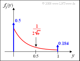
PDF after amplification and boundary

(3)  The fourth-order central moment is  $\mu_4 = m_4 = 4!/2^4 = 1.5$.

  • From this follows for the kurtosis:
$$K_{x}=\frac{ \mu_{\rm 4}}{ \sigma_{\it x}^{4}}=\frac{1.5}{0.25}\hspace{0.15cm}\underline{=\rm 6}.$$


(4)  Using the result from  (1)  we get:

$${\rm Pr}( x> 0.5)=\int_{0.5}^{\infty}{\rm e}^{- 2 x}\,{\rm d}x=\frac{\rm 1}{\rm 2\rm e}\hspace{0.15cm}\underline{=\rm 18.4\%}.$$


(5)  Correct are the  solutions 1 and 3:

  • The PDF  $f_y(y)$  involves a Dirac delta function at the point  $y= 0$  with weight  ${\rm Pr}(x < 0) = 0.5$.
  • In addition,  another Dirac delta function at  $y= 1$  with weight  ${\rm Pr}(x > 0.5) = 0.184$.


(6)  The signal range  $0 \le x \le 0.5$  is linearly mapped to the range  $0 \le y \le 1$  at the output.

  • The derivative of the characteristic curve is constantly equal to $2$  (amplification). From this one obtains:
$$f_y(y)=\frac{f_x(x)}{|g'(x)|}\Bigg|_{x=h(y)}=\frac{\rm e^{-\rm 2\it x}}{\rm 2}\Bigg|_{\it x={\it y}/{\rm 2}}=0.5 \cdot {\rm e^{\it -y}} .$$
  • For  $y= 0.5$  accordingly,  the continuous PDF component is
$$f_y(y = 0.5)\hspace{0.15cm}\underline{\approx 0.304}.$$


(7)  For the mean value of the random variable  $y$  holds:

$$m_y=\frac{1}{\rm 2\rm e} \cdot 1 +\int_{\rm 0}^{\rm 1}\frac{\it y}{\rm 2}\cdot \rm e^{\it -y}\, \rm d \it y=\frac{\rm 1}{\rm 2\rm e}{\rm +}\frac{\rm 1}{\rm 2}-\frac{\rm 1}{\rm e}=\frac{\rm 1}{\rm 2}-\frac{\rm 1}{\rm 2 e}\hspace{0.15cm}\underline{=\rm 0.316}.$$
  • The first term is from the Dirac delta at  $y= 1$,  the second from the continuous PDF component.