Difference between revisions of "Aufgaben:Exercise 5.1Z: Sampling of Harmonic Oscillations"
m (Text replacement - "Time Discrete" to "Discrete-Time") |
|||
| (10 intermediate revisions by 4 users not shown) | |||
| Line 3: | Line 3: | ||
}} | }} | ||
| − | [[File:P_ID1129__Sig_Z_5_1.png|right|frame| | + | [[File:P_ID1129__Sig_Z_5_1.png|right|frame|Three harmonic oscillations of equal frequency $f_0$ and equal amplitude $A$]] |
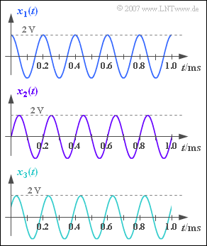
| − | + | We consider three harmonic oscillations with the same frequency and the same amplitude: | |
:$$x_1(t) = A \cdot \cos (2 \pi \cdot f_0 \cdot t) \hspace{0.05cm}, $$ | :$$x_1(t) = A \cdot \cos (2 \pi \cdot f_0 \cdot t) \hspace{0.05cm}, $$ | ||
:$$ x_2(t) = A \cdot \sin (2 \pi \cdot f_0 \cdot t) \hspace{0.05cm}, $$ | :$$ x_2(t) = A \cdot \sin (2 \pi \cdot f_0 \cdot t) \hspace{0.05cm}, $$ | ||
:$$ x_3(t) = A \cdot \cos (2 \pi \cdot f_0 \cdot t - 60^{\circ}) \hspace{0.05cm}.$$ | :$$ x_3(t) = A \cdot \cos (2 \pi \cdot f_0 \cdot t - 60^{\circ}) \hspace{0.05cm}.$$ | ||
| − | + | The oscillation parameters $f_0$ and $A$ can be taken from the graph. | |
| − | + | It is assumed that the signals are sampled equidistantly at times $\nu \cdot T_{\rm A}$ whereby the parameter values $T_{\rm A} = 80 \ µ \text{s}$ and $T_{\rm A} = 100 \ µ \text{s}$ are to be analyzed. | |
| − | + | The signal reconstruction at the receiver takes place through a low-pass filter $H(f)$, which forms the signal $y_{\rm A}(t) = x_{\rm A}(t)$ from the sampled signal $y(t)$ . It applies: | |
:$$H(f) = \left\{ \begin{array}{c} 1 \\ 0.5 \\ | :$$H(f) = \left\{ \begin{array}{c} 1 \\ 0.5 \\ | ||
0 \\ \end{array} \right.\quad | 0 \\ \end{array} \right.\quad | ||
| Line 22: | Line 22: | ||
|f| > f_{\rm G} \hspace{0.05cm}, \\ | |f| > f_{\rm G} \hspace{0.05cm}, \\ | ||
\end{array}$$ | \end{array}$$ | ||
| − | + | Here $f_{\rm G}$ indicates the cut-off frequency of the rectangular low-pass filter. For this shall apply: | |
:$$f_{\rm G} = \frac{1}{ 2 \cdot T_{\rm A}}\hspace{0.05cm}.$$ | :$$f_{\rm G} = \frac{1}{ 2 \cdot T_{\rm A}}\hspace{0.05cm}.$$ | ||
| − | + | The sampling theorem is fulfilled if $y(t) = x(t)$ holds. | |
| Line 31: | Line 31: | ||
| − | '' | + | ''Hints:'' |
| − | * | + | *This task belongs to the chapter [[Signal_Representation/Time_Discrete_Signal_Representation|Discrete-Time Signal Representation]]. |
| − | * | + | *There is an interactive applet for the topic dealt with here: [[Applets:Sampling_of_Analog_Signals_and_Signal_Reconstruction|Sampling of Analog Signals and Signal Reconstruction]] |
| − | === | + | |
| + | ===Questions=== | ||
<quiz display=simple> | <quiz display=simple> | ||
| − | { | + | {What are the amplitude and frequency of the signals $x_1(t)$, $x_2(t)$ and $x_3(t)$? |
|type="{}"} | |type="{}"} | ||
$A \hspace{0.25cm} = \ $ { 2 3% } $\text{V}$ | $A \hspace{0.25cm} = \ $ { 2 3% } $\text{V}$ | ||
| Line 46: | Line 47: | ||
| − | { | + | {For which input signals is the sampling theorem satisfied ⇒ $y(t) = x(t)$, when $\underline{T_{\rm A} = 80 \ {\rm µ} \text{s}}$ ? |
|type="[]"} | |type="[]"} | ||
+ $x_1(t)$, | + $x_1(t)$, | ||
| Line 53: | Line 54: | ||
| − | { | + | {What is the reconstructed signal $y_1(t) = A_1 \cdot \cos (2\pi f_0 t – \varphi_1)$ with the sampling distance $\underline{T_{\rm A} = 100 \ {\rm µ} \text{s}}$? Interpret the result. |
|type="{}"} | |type="{}"} | ||
$A_1\hspace{0.2cm} = \ ${ 2 3% } $\text{V}$ | $A_1\hspace{0.2cm} = \ ${ 2 3% } $\text{V}$ | ||
| − | $\varphi_1\hspace{0.2cm} = \ $ { 0. } $\text{ | + | $\varphi_1\hspace{0.2cm} = \ $ { 0. } $\text{Deg}$ |
| − | { | + | {What is the amplitude $A_2$ of the reconstructed signal $y_2(t)$, when the sinusoidal signal $x_2(t)$ is present? Let $\underline{T_{\rm A} = 100 \ {\rm µ} \text{s}}$ still apply. |
|type="{}"} | |type="{}"} | ||
$A_2\hspace{0.2cm} = \ $ { 0. } $\text{V}$ | $A_2\hspace{0.2cm} = \ $ { 0. } $\text{V}$ | ||
| − | { | + | {What is the amplitude $A_3$ of the reconstructed signal $y_3(t)$, when the signal $x_3(t)$ is present? $\underline{T_{\rm A} = 100 \ {\rm µ} \text{s}}$ is still valid. |
|type="{}"} | |type="{}"} | ||
$A_3\hspace{0.2cm} = \ $ { 1 3% } $\text{V}$ | $A_3\hspace{0.2cm} = \ $ { 1 3% } $\text{V}$ | ||
| Line 72: | Line 73: | ||
</quiz> | </quiz> | ||
| − | === | + | ===Solution=== |
{{ML-Kopf}} | {{ML-Kopf}} | ||
| − | '''(1)''' | + | '''(1)''' The graph shows the amplitude $\underline{A = 2\ \text{V}}$ and the period $T_0 = 0.2 \ \text{ms}$. |
| − | * | + | *This results in the signal frequency $f_0 = 1/T_0 \; \underline{= 5 \ \text{kHz}}$. |
| − | '''(2)''' | + | '''(2)''' <u>All proposed solutions</u> are correct: |
| − | * | + | *The sampling rate here is $f_{\rm A} = 1/T_{\rm A} = 12.5 \ \text{kHz}$. |
| − | * | + | *This value is greater than $2 \cdot f_0 = 10 \ \text{kHz}$. |
| − | * | + | *Thus the sampling theorem is fulfilled independently of the phase and $y(t) = x(t)$ always applies. |
| − | [[File:P_ID1130__Sig_Z_5_1_c.png|right|frame| | + | [[File:P_ID1130__Sig_Z_5_1_c.png|right|frame|Spectrum $X_{\rm A}(f)$ of the sampled signal – real part and imaginary part]] |
| − | '''(3)''' | + | '''(3)''' The sampling rate is now $f_{\rm A} = 2 \cdot f_0 = 10 \ \text{kHz}$. |
| − | * | + | *Only in the special case of the cosine signal the sampling theorem is satisfied, and it holds: |
:$$y_1(t) = x_1(t) ⇒ A_1 \; \underline{=2 \ \text{V}} \text{ und }\varphi_1 \; \underline{= 0}.$$ | :$$y_1(t) = x_1(t) ⇒ A_1 \; \underline{=2 \ \text{V}} \text{ und }\varphi_1 \; \underline{= 0}.$$ | ||
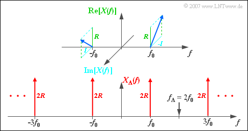
| − | + | This result is now to be derived mathematically, whereby a phase $\varphi$ in the input signal is already taken into account with regard to the remaining subtasks: | |
| − | |||
:$$x(t) = A \cdot \cos (2 \pi \cdot f_0 \cdot t - \varphi) | :$$x(t) = A \cdot \cos (2 \pi \cdot f_0 \cdot t - \varphi) | ||
\hspace{0.05cm}.$$ | \hspace{0.05cm}.$$ | ||
| − | * | + | *Then, for the spectral function sketched in the graph above: |
:$$X(f) = {A}/{2} \hspace{0.05cm} \cdot \hspace{0.05cm} {\rm e}^{{\rm j} \hspace{0.05cm} | :$$X(f) = {A}/{2} \hspace{0.05cm} \cdot \hspace{0.05cm} {\rm e}^{{\rm j} \hspace{0.05cm} | ||
\cdot \hspace{0.05cm} \varphi} \cdot \delta | \cdot \hspace{0.05cm} \varphi} \cdot \delta | ||
| Line 99: | Line 99: | ||
\cdot \hspace{0.05cm} \varphi} \cdot \delta | \cdot \hspace{0.05cm} \varphi} \cdot \delta | ||
(f- f_{\rm 0} )\hspace{0.05cm}.$$ | (f- f_{\rm 0} )\hspace{0.05cm}.$$ | ||
| − | * | + | *With the abbreviations |
:$$R = {A}/{2} \hspace{0.05cm} \cdot \hspace{0.05cm} | :$$R = {A}/{2} \hspace{0.05cm} \cdot \hspace{0.05cm} | ||
| − | \cos(\varphi) \hspace{0.5cm}{\rm | + | \cos(\varphi) \hspace{0.5cm}{\rm and} \hspace{0.5cm}I ={A}/{2} \hspace{0.05cm} \cdot |
\hspace{0.05cm} \sin(\varphi)$$ | \hspace{0.05cm} \sin(\varphi)$$ | ||
| − | : | + | :can also be written for this: |
:$$X(f) = (R + {\rm j} \cdot I) \cdot \delta | :$$X(f) = (R + {\rm j} \cdot I) \cdot \delta | ||
(f+ f_{\rm 0} ) + (R - {\rm j} \cdot I) \cdot \delta | (f+ f_{\rm 0} ) + (R - {\rm j} \cdot I) \cdot \delta | ||
(f- f_{\rm 0} )\hspace{0.05cm}.$$ | (f- f_{\rm 0} )\hspace{0.05cm}.$$ | ||
| − | * | + | *The spectrum of the signal $x_{\rm A}(t)$ sampled with $f_{\rm A} = 2f_0$ is thus: |
:$$X_{\rm A}(f) = \sum_{\mu = - \infty }^{+\infty} X (f- \mu \cdot f_{\rm A} | :$$X_{\rm A}(f) = \sum_{\mu = - \infty }^{+\infty} X (f- \mu \cdot f_{\rm A} | ||
)= \sum_{\mu = - \infty }^{+\infty} X (f- 2\mu \cdot f_{\rm 0} | )= \sum_{\mu = - \infty }^{+\infty} X (f- 2\mu \cdot f_{\rm 0} | ||
)\hspace{0.05cm}.$$ | )\hspace{0.05cm}.$$ | ||
| − | :* | + | :*The bottom graph shows that $X_{\rm A}(f)$ consists of Dirac functions at $\pm f_0$, $\pm 3f_0$, $\pm 5f_0$, and so on. |
| − | :* | + | :*All weights are purely real and equal to $2 \cdot R$. |
| − | :* | + | :*The imaginary parts of the periodically continued spectrum cancel out. |
| − | * | + | *If one further takes into account the rectangular low-pass filter whose cut-off frequency lies exactly at $f_{\rm G} = f_0$, as well as $H(f_{\rm G}) = 0.5$, one obtains for the spectrum after signal reconstruction: |
:$$Y(f) = R \cdot \delta | :$$Y(f) = R \cdot \delta | ||
(f+ f_{\rm 0} ) + R \cdot \delta | (f+ f_{\rm 0} ) + R \cdot \delta | ||
| Line 121: | Line 121: | ||
\cos(\varphi)\hspace{0.05cm}.$$ | \cos(\varphi)\hspace{0.05cm}.$$ | ||
| − | * | + | *The inverse Fourier transformation leads to |
| − | [[File:P_ID1131__Sig_Z_5_1_d.png|right|frame| | + | [[File:P_ID1131__Sig_Z_5_1_d.png|right|frame|Reconstruction of the sampled sine signal]] |
:$$y(t) = A \cdot \cos (\varphi)\cdot \cos (2 \pi \cdot f_0 \cdot t ) | :$$y(t) = A \cdot \cos (\varphi)\cdot \cos (2 \pi \cdot f_0 \cdot t ) | ||
\hspace{0.05cm}.$$ | \hspace{0.05cm}.$$ | ||
| − | * | + | *Thus, a cosine-shaped progression results independent of the input phase $\varphi$ . |
| − | * | + | *If $\varphi = 0$ as with the signal $x_1(t)$, the amplitude of the output signal is also equal to $A$. |
| − | '''(4)''' | + | '''(4)''' The sine signal has the phase $90^\circ$. |
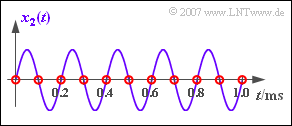
| − | * | + | *From this follows directly $y_2(t) = 0$ ⇒ amplitude $\underline{A_2 = 0}$. |
| − | * | + | *This result becomes understandable if you look at the samples in the graph. |
| − | * | + | *All samples (red circles) are zero, so there can be no signal even after the filter. |
| − | [[File:P_ID1133__Sig_Z_5_1_e.png|right|frame| | + | [[File:P_ID1133__Sig_Z_5_1_e.png|right|frame|Reconstruction of a harmonic oscillation with $60^\circ$ phase]] |
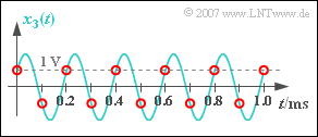
| − | '''(5)''' | + | '''(5)''' Despite ⇒ $\varphi = 60^\circ$ gilt $\varphi_3 = 0$ ⇒ the reconstructed signal $y_3(t)$ is cosine-shaped, too. |
| + | *The amplitude is equal to | ||
:$$A_3 = A \cdot \cos (60^{\circ})= {A}/{2} \hspace{0.15 cm}\underline{= 1\,{\rm V}} | :$$A_3 = A \cdot \cos (60^{\circ})= {A}/{2} \hspace{0.15 cm}\underline{= 1\,{\rm V}} | ||
\hspace{0.05cm}.$$ | \hspace{0.05cm}.$$ | ||
| − | * | + | *If you look at the samples drawn in red in the graph, you will admit that you as a "signal reconstructor" would not make any other decision than the low-pass. |
| − | * | + | *Because, you don't know the turquoise curve. |
{{ML-Fuß}} | {{ML-Fuß}} | ||
__NOEDITSECTION__ | __NOEDITSECTION__ | ||
| − | [[Category: | + | [[Category:Signal Representation: Exercises|^5.1 Discrete-Time Signal Representation^]] |
Latest revision as of 11:03, 11 October 2021
We consider three harmonic oscillations with the same frequency and the same amplitude:
- $$x_1(t) = A \cdot \cos (2 \pi \cdot f_0 \cdot t) \hspace{0.05cm}, $$
- $$ x_2(t) = A \cdot \sin (2 \pi \cdot f_0 \cdot t) \hspace{0.05cm}, $$
- $$ x_3(t) = A \cdot \cos (2 \pi \cdot f_0 \cdot t - 60^{\circ}) \hspace{0.05cm}.$$
The oscillation parameters $f_0$ and $A$ can be taken from the graph.
It is assumed that the signals are sampled equidistantly at times $\nu \cdot T_{\rm A}$ whereby the parameter values $T_{\rm A} = 80 \ µ \text{s}$ and $T_{\rm A} = 100 \ µ \text{s}$ are to be analyzed.
The signal reconstruction at the receiver takes place through a low-pass filter $H(f)$, which forms the signal $y_{\rm A}(t) = x_{\rm A}(t)$ from the sampled signal $y(t)$ . It applies:
- $$H(f) = \left\{ \begin{array}{c} 1 \\ 0.5 \\ 0 \\ \end{array} \right.\quad \begin{array}{*{5}c} {\rm{{\rm{f\ddot{u}r}}}} \\ {\rm{{\rm{f\ddot{u}r}}}} \\ {\rm{{\rm{f\ddot{u}r}}}} \\ \end{array}\begin{array}{*{5}c} |f| < f_{\rm G} \hspace{0.05cm}, \\ |f| = f_{\rm G} \hspace{0.05cm}, \\ |f| > f_{\rm G} \hspace{0.05cm}, \\ \end{array}$$
Here $f_{\rm G}$ indicates the cut-off frequency of the rectangular low-pass filter. For this shall apply:
- $$f_{\rm G} = \frac{1}{ 2 \cdot T_{\rm A}}\hspace{0.05cm}.$$
The sampling theorem is fulfilled if $y(t) = x(t)$ holds.
Hints:
- This task belongs to the chapter Discrete-Time Signal Representation.
- There is an interactive applet for the topic dealt with here: Sampling of Analog Signals and Signal Reconstruction
Questions
Solution
- This results in the signal frequency $f_0 = 1/T_0 \; \underline{= 5 \ \text{kHz}}$.
(2) All proposed solutions are correct:
- The sampling rate here is $f_{\rm A} = 1/T_{\rm A} = 12.5 \ \text{kHz}$.
- This value is greater than $2 \cdot f_0 = 10 \ \text{kHz}$.
- Thus the sampling theorem is fulfilled independently of the phase and $y(t) = x(t)$ always applies.
(3) The sampling rate is now $f_{\rm A} = 2 \cdot f_0 = 10 \ \text{kHz}$.
- Only in the special case of the cosine signal the sampling theorem is satisfied, and it holds:
- $$y_1(t) = x_1(t) ⇒ A_1 \; \underline{=2 \ \text{V}} \text{ und }\varphi_1 \; \underline{= 0}.$$
This result is now to be derived mathematically, whereby a phase $\varphi$ in the input signal is already taken into account with regard to the remaining subtasks:
- $$x(t) = A \cdot \cos (2 \pi \cdot f_0 \cdot t - \varphi) \hspace{0.05cm}.$$
- Then, for the spectral function sketched in the graph above:
- $$X(f) = {A}/{2} \hspace{0.05cm} \cdot \hspace{0.05cm} {\rm e}^{{\rm j} \hspace{0.05cm} \cdot \hspace{0.05cm} \varphi} \cdot \delta (f+ f_{\rm 0} ) + {A}/{2} \hspace{0.05cm} \cdot \hspace{0.05cm} {\rm e}^{-{\rm j} \hspace{0.05cm} \cdot \hspace{0.05cm} \varphi} \cdot \delta (f- f_{\rm 0} )\hspace{0.05cm}.$$
- With the abbreviations
- $$R = {A}/{2} \hspace{0.05cm} \cdot \hspace{0.05cm} \cos(\varphi) \hspace{0.5cm}{\rm and} \hspace{0.5cm}I ={A}/{2} \hspace{0.05cm} \cdot \hspace{0.05cm} \sin(\varphi)$$
- can also be written for this:
- $$X(f) = (R + {\rm j} \cdot I) \cdot \delta (f+ f_{\rm 0} ) + (R - {\rm j} \cdot I) \cdot \delta (f- f_{\rm 0} )\hspace{0.05cm}.$$
- The spectrum of the signal $x_{\rm A}(t)$ sampled with $f_{\rm A} = 2f_0$ is thus:
- $$X_{\rm A}(f) = \sum_{\mu = - \infty }^{+\infty} X (f- \mu \cdot f_{\rm A}
)= \sum_{\mu = - \infty }^{+\infty} X (f- 2\mu \cdot f_{\rm 0}
)\hspace{0.05cm}.$$
- The bottom graph shows that $X_{\rm A}(f)$ consists of Dirac functions at $\pm f_0$, $\pm 3f_0$, $\pm 5f_0$, and so on.
- All weights are purely real and equal to $2 \cdot R$.
- The imaginary parts of the periodically continued spectrum cancel out.
- If one further takes into account the rectangular low-pass filter whose cut-off frequency lies exactly at $f_{\rm G} = f_0$, as well as $H(f_{\rm G}) = 0.5$, one obtains for the spectrum after signal reconstruction:
- $$Y(f) = R \cdot \delta (f+ f_{\rm 0} ) + R \cdot \delta (f- f_{\rm 0} )\hspace{0.05cm}, \hspace{0.5cm} R = {A}/{2} \hspace{0.05cm} \cdot \hspace{0.05cm} \cos(\varphi)\hspace{0.05cm}.$$
- The inverse Fourier transformation leads to
- $$y(t) = A \cdot \cos (\varphi)\cdot \cos (2 \pi \cdot f_0 \cdot t ) \hspace{0.05cm}.$$
- Thus, a cosine-shaped progression results independent of the input phase $\varphi$ .
- If $\varphi = 0$ as with the signal $x_1(t)$, the amplitude of the output signal is also equal to $A$.
(4) The sine signal has the phase $90^\circ$.
- From this follows directly $y_2(t) = 0$ ⇒ amplitude $\underline{A_2 = 0}$.
- This result becomes understandable if you look at the samples in the graph.
- All samples (red circles) are zero, so there can be no signal even after the filter.
(5) Despite ⇒ $\varphi = 60^\circ$ gilt $\varphi_3 = 0$ ⇒ the reconstructed signal $y_3(t)$ is cosine-shaped, too.
- The amplitude is equal to
- $$A_3 = A \cdot \cos (60^{\circ})= {A}/{2} \hspace{0.15 cm}\underline{= 1\,{\rm V}} \hspace{0.05cm}.$$
- If you look at the samples drawn in red in the graph, you will admit that you as a "signal reconstructor" would not make any other decision than the low-pass.
- Because, you don't know the turquoise curve.


