Difference between revisions of "Applets:Linear Distortions of Periodic Signals"
| (8 intermediate revisions by 3 users not shown) | |||
| Line 1: | Line 1: | ||
| − | {{ | + | {{LntAppletLink|physAnSignal_en}} [https://en.lntwww.de/Applets:Physical_Signal_%26_Analytic_Signal '''English Applet with English WIKI description'''] |
==Applet Description== | ==Applet Description== | ||
| Line 14: | Line 14: | ||
| − | The next block in the model above is ''Matching'': The output signal $y(t)$ is adjusted in amplitude and phase with equal | + | The next block in the model above is ''Matching'': The output signal $y(t)$ is adjusted in amplitude and phase with equal variables $k_{\rm M}$ and $\tau_{\rm M}$ for all frequencies which means that this is not a frequency-dependent equalization. Using the signal $z(t)$, one can differentiate between: |
| − | *attenuation distortion and frequency– | + | *attenuation distortion and frequency–independent attenuation, as well as |
| − | *phase distortion and frequency– | + | *phase distortion and frequency–independent delay. |
The ''Distortion Power'' $P_{\rm D}$ is used to measure the strength of the linear distortion and is defined as: | The ''Distortion Power'' $P_{\rm D}$ is used to measure the strength of the linear distortion and is defined as: | ||
:$$P_{\rm D} = \min_{k_{\rm M}, \ \tau_{\rm M}} P_\varepsilon.$$ | :$$P_{\rm D} = \min_{k_{\rm M}, \ \tau_{\rm M}} P_\varepsilon.$$ | ||
| − | |||
| − | |||
| Line 46: | Line 44: | ||
*'''Nonlinear distortions''' occur, if at all times $t$ the nonlinear correlation $y = g(x) \ne {\rm const.} \cdot x$ exists between the signal values $x = x(t)$ at the input and $y = y(t)$ at the output, whereby $y = g(x)$ is defined as the system's nonlinear characteristic. By creating a cosine signal at the input with frequency $f_0$ the output signal includes $f_0$, as well as multiple harmonic waves. We conclude that new frequencies arise through nonlinear distortion. | *'''Nonlinear distortions''' occur, if at all times $t$ the nonlinear correlation $y = g(x) \ne {\rm const.} \cdot x$ exists between the signal values $x = x(t)$ at the input and $y = y(t)$ at the output, whereby $y = g(x)$ is defined as the system's nonlinear characteristic. By creating a cosine signal at the input with frequency $f_0$ the output signal includes $f_0$, as well as multiple harmonic waves. We conclude that new frequencies arise through nonlinear distortion. | ||
| − | [[File: | + | [[File:EN_LZI_T_2_2_S3_v2.png|center|frame|For clarification of nonlinear distortions |class=fit]] |
[[File:P_ID899__LZI_T_2_3_S1_neu.png|right |frame| Description of a linear system|class=fit]] | [[File:P_ID899__LZI_T_2_3_S1_neu.png|right |frame| Description of a linear system|class=fit]] | ||
| Line 69: | Line 67: | ||
*The '''phase function''' $b(f)$ indicates the negative frequency–dependent angle of $H(f)$ in the complex plane based on the real axis: | *The '''phase function''' $b(f)$ indicates the negative frequency–dependent angle of $H(f)$ in the complex plane based on the real axis: | ||
:$$b(f) = - {\rm arc} \hspace{0.1cm}H(f) \hspace{0.2cm}{\rm in | :$$b(f) = - {\rm arc} \hspace{0.1cm}H(f) \hspace{0.2cm}{\rm in | ||
| − | \hspace{0.1cm} | + | \hspace{0.1cm}Radians \hspace{0.1cm}(rad)}.$$ |
| Line 95: | Line 93: | ||
The frequency response of a realizable high–pass (HP) of order $N$ is: | The frequency response of a realizable high–pass (HP) of order $N$ is: | ||
:$$H(f) = \left [\frac{ {\rm j}\cdot f/f_0 }{1 + {\rm j}\cdot f/f_0 }\right ]^N\hspace{0.05cm}.$$ | :$$H(f) = \left [\frac{ {\rm j}\cdot f/f_0 }{1 + {\rm j}\cdot f/f_0 }\right ]^N\hspace{0.05cm}.$$ | ||
| − | For example the LC high pass is a first order high pass. Consequently we can obtain | + | For example the LC high-pass is a first order high-pass. Consequently we can obtain |
*the attenuation function: | *the attenuation function: | ||
:$$a(f) =N/2 \cdot \ln [1+( f_0/f)^2] \hspace{0.05cm},$$ | :$$a(f) =N/2 \cdot \ln [1+( f_0/f)^2] \hspace{0.05cm},$$ | ||
| Line 111: | Line 109: | ||
{{GraueBox|TEXT= | {{GraueBox|TEXT= | ||
$\text{Example:}$ | $\text{Example:}$ | ||
| − | This graphic shows the phase function $b(f)$ with the | + | This graphic shows the phase function $b(f)$ with the cutoff frequency $f_0 = 1\ \rm kHz$ and order $N=1$ |
* of a low–pass (green curve), | * of a low–pass (green curve), | ||
* of a high–pass (violet curve). | * of a high–pass (violet curve). | ||
| Line 129: | Line 127: | ||
| − | ''Remark:'' The shown signals were created using the interactive applet [[Applets:Kausale_Systeme_-_Laplacetransformation|Causal systems – Laplace transform]]. }} | + | ''Remark:'' The shown signals were created using the interactive applet [[Applets:Kausale_Systeme_-_Laplacetransformation|"Causal systems – Laplace transform"]]. }} |
=== Attenuation and Phase Distortions === | === Attenuation and Phase Distortions === | ||
| Line 165: | Line 163: | ||
*An exercise description is displayed. | *An exercise description is displayed. | ||
*Parameter values are adjusted to the respective exercises. | *Parameter values are adjusted to the respective exercises. | ||
| − | *Click | + | *Click "Hide solution" to display the solution. |
| − | Number | + | Number "0" is a "Reset" button: |
*Sets parameters to initial values (when loading the page). | *Sets parameters to initial values (when loading the page). | ||
| − | *Displays a | + | *Displays a "Reset text" to describe the applet further. |
| Line 295: | Line 293: | ||
'''(C)''' Selction of channel parameters per slider: Dämpfungsfaktoren und Phasenlaufzeiten | '''(C)''' Selction of channel parameters per slider: Dämpfungsfaktoren und Phasenlaufzeiten | ||
| − | '''(D)''' Selection of channel parameters for High and Low pass: Order$n$, | + | '''(D)''' Selection of channel parameters for High and Low pass: Order$n$, cutoff frequency $f_0$ |
'''(E)''' Selection of matching parameters $k_{\rm M}$ and $\varphi_{\rm M}$ | '''(E)''' Selection of matching parameters $k_{\rm M}$ and $\varphi_{\rm M}$ | ||
| Line 315: | Line 313: | ||
'''(M)''' Variation possibilities for the graphic display | '''(M)''' Variation possibilities for the graphic display | ||
| − | $\hspace{1.5cm}$Zoom–functions | + | $\hspace{1.5cm}$Zoom–functions "$+$" (scale up), "$-$" (scale down) und $\rm o$ (reset) |
| − | $\hspace{1.5cm}$Move with | + | $\hspace{1.5cm}$Move with "$\leftarrow$" (section to the left, ordinate to the right), "$\uparrow$" "$\downarrow$" und "$\rightarrow$" |
$\hspace{1.5cm}$'''Other options'': | $\hspace{1.5cm}$'''Other options'': | ||
| Line 327: | Line 325: | ||
==About the Authors== | ==About the Authors== | ||
This interactive calculation was designed and realized at the [http://www.lnt.ei.tum.de/startseite Lehrstuhl für Nachrichtentechnik] of the [https://www.tum.de/ Technische Universität München]. | This interactive calculation was designed and realized at the [http://www.lnt.ei.tum.de/startseite Lehrstuhl für Nachrichtentechnik] of the [https://www.tum.de/ Technische Universität München]. | ||
| − | *The original version was created in 2005 by [[Biographies_and_Bibliographies/An_LNTwww_beteiligte_Studierende#Bettina_Hirner_.28Diplomarbeit_LB_2005.29|Bettina Hirner]] as part of her Diploma thesis using | + | *The original version was created in 2005 by [[Biographies_and_Bibliographies/An_LNTwww_beteiligte_Studierende#Bettina_Hirner_.28Diplomarbeit_LB_2005.29|Bettina Hirner]] as part of her Diploma thesis using "FlashMX–Actionscript" (Supervisor: [[Biographies_and_Bibliographies/An_LNTwww_beteiligte_Mitarbeiter_und_Dozenten#Prof._Dr.-Ing._habil._G.C3.BCnter_S.C3.B6der_.28am_LNT_seit_1974.29|Günter Söder]] ). |
| − | *In 2018 this Applet was redesigned and updated to | + | *In 2018 this Applet was redesigned and updated to "HTML5" by [[Biographies_and_Bibliographies/An_LNTwww_beteiligte_Studierende#Jimmy_He_.28Bachelorarbeit_2018.29|Jimmy He]] as part of his Bachelor's thesis (Supervisor: [[Biographies_and_Bibliographies/Beteiligte_der_Professur_Leitungsgebundene_%C3%9Cbertragungstechnik#Tasn.C3.A1d_Kernetzky.2C_M.Sc._.28bei_L.C3.9CT_seit_2014.29|Tasnád Kernetzky]]) . |
==Once again: Open Applet in new Tab== | ==Once again: Open Applet in new Tab== | ||
{{LntAppletLinkEn|linDistortions_en}} [https://www.lntwww.de/Applets:Lineare_Verzerrungen_periodischer_Signale '''English Applet with German WIKI description'''] | {{LntAppletLinkEn|linDistortions_en}} [https://www.lntwww.de/Applets:Lineare_Verzerrungen_periodischer_Signale '''English Applet with German WIKI description'''] | ||
Latest revision as of 17:16, 13 April 2023
Open Applet in a new tab English Applet with English WIKI description
Contents
Applet Description
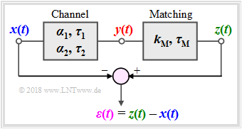
This applet illustrates the effects of linear distortions (attenuation distortions and phase distortions) with
- the input signal $x(t)$ ⇒ power $P_x$:
- $$x(t) = x_1(t) + x_2(t) = A_1\cdot \cos\left(2\pi f_1\cdot t- \varphi_1\right)+A_2\cdot \cos\left(2\pi f_2\cdot t- \varphi_2\right), $$
- the output signal $y(t)$ ⇒ power $P_y$:
- $$y(t) = \alpha_1 \cdot x_1(t-\tau_1) + \alpha_2 \cdot x_2(t-\tau_2),$$
- the matched output signal $z(t)$ ⇒ power $P_z$:
- $$z(t) = k_{\rm M} \cdot y(t-\tau_{\rm M}) + \alpha_2 \cdot x_2(t-\tau_2),$$
- the difference signal $\varepsilon(t) = z(t) - x(t)$ ⇒ power $P_\varepsilon$.
The next block in the model above is Matching: The output signal $y(t)$ is adjusted in amplitude and phase with equal variables $k_{\rm M}$ and $\tau_{\rm M}$ for all frequencies which means that this is not a frequency-dependent equalization. Using the signal $z(t)$, one can differentiate between:
- attenuation distortion and frequency–independent attenuation, as well as
- phase distortion and frequency–independent delay.
The Distortion Power $P_{\rm D}$ is used to measure the strength of the linear distortion and is defined as:
- $$P_{\rm D} = \min_{k_{\rm M}, \ \tau_{\rm M}} P_\varepsilon.$$
Theoretical Background
Distortions refer to generally unwanted alterations of a message signal through a transmission system. Together with the strong stochastic effects (noise, crosstalk, etc.), they are a crucial limitation for the quality and rate of transmission.
Just as the intensity of noise can be assessed through
- the Noise Power $P_{\rm N}$ and
- the Signal–to–Noise Ratio (SNR) $\rho_{\rm N}$,
distortions can be quantified through
- the Distortion Power $P_{\rm D}$ and
- the Signal–to–Distortion Ratio (SDR)
- $$\rho_{\rm D}=\frac{\rm Signal \ Power}{\rm Distortion \ Power} = \frac{P_x}{P_{\rm D} }.$$
Linear and Nonlinear Distortions
A distinction is made between linear and nonlinear distortions:
- Nonlinear distortions occur, if at all times $t$ the nonlinear correlation $y = g(x) \ne {\rm const.} \cdot x$ exists between the signal values $x = x(t)$ at the input and $y = y(t)$ at the output, whereby $y = g(x)$ is defined as the system's nonlinear characteristic. By creating a cosine signal at the input with frequency $f_0$ the output signal includes $f_0$, as well as multiple harmonic waves. We conclude that new frequencies arise through nonlinear distortion.
- Linear distortions occur, if the transmission channel is characterized by a frequency response $H(f) \ne \rm const.$ Various frequencies are attenuated and delayed differently. Characteristic of this is that although frequencies can disappear (for example, through a low–pass, a high–pass, or a band–pass), no new frequencies can arise.
In this applet only linear distortions are considered.
Description Forms for the Frequency Response
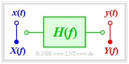
The generally complex valued frequency response can be represented as follows:
- $$H(f) = |H(f)| \cdot {\rm e}^{-{\rm j} \hspace{0.05cm} \cdot \hspace{0.05cm} b(f)} = {\rm e}^{-a(f)}\cdot {\rm e}^{-{\rm j} \hspace{0.05cm} \cdot \hspace{0.05cm} b(f)}.$$
This results in the following description variables:
- The absolute value $|H(f)|$ is called amplitude response and in logarithmic form attenuation function:
- $$a(f) = - \ln |H(f)|\hspace{0.2cm}{\rm in \hspace{0.1cm}Neper \hspace{0.1cm}(Np) } = - 20 \cdot \lg |H(f)|\hspace{0.2cm}{\rm in \hspace{0.1cm}Decibel \hspace{0.1cm}(dB) }.$$
- The phase function $b(f)$ indicates the negative frequency–dependent angle of $H(f)$ in the complex plane based on the real axis:
- $$b(f) = - {\rm arc} \hspace{0.1cm}H(f) \hspace{0.2cm}{\rm in \hspace{0.1cm}Radians \hspace{0.1cm}(rad)}.$$
Low–pass of Order N
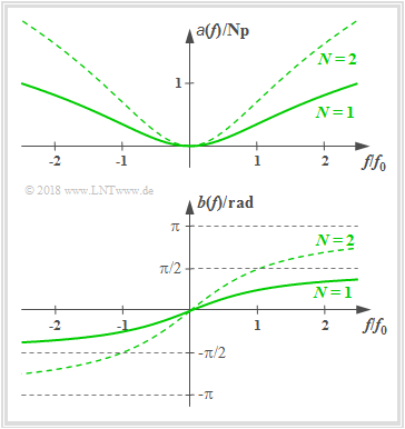
The frequency response of a realizable low–pass (LP) of order $N$ is:
- $$H(f) = \left [\frac{1}{1 + {\rm j}\cdot f/f_0 }\right ]^N\hspace{0.05cm}.$$
For example the RC low–pass is a first order low–pass. Consequently we can obtain
- the attenuation function:
- $$a(f) =N/2 \cdot \ln [1+( f/f_0)^2] \hspace{0.05cm},$$
- the phase function:
- $$b(f) =N \cdot \arctan( f/f_0) \hspace{0.05cm},$$
- the attenuation factor for the frequency $f=f_i$:
- $$\alpha_i =|H(f = f_i)| = [1+( f_i/f_0)^2]^{-N/2}$$
- $$\Rightarrow \hspace{0.3cm} x(t)= A_i\cdot \cos(2\pi f_i t) \hspace{0.1cm}\rightarrow \hspace{0.1cm} y(t)= \alpha_i \cdot A_i\cdot \cos(2\pi f_i t)\hspace{0.05cm},$$
- the phase delay for the frequency $f=f_i$:
- $$\tau_i =\frac{b(f_i)}{2 \pi f_i} = \frac{N \cdot \arctan( f_i/f_0)}{2 \pi f_i}$$
- $$\Rightarrow \hspace{0.3cm} x(t)= A_i\cdot \cos(2\pi f_i t) \hspace{0.1cm}\rightarrow \hspace{0.1cm} y(t)=A_i\cdot \cos(2\pi f_i (t- \tau_i))\hspace{0.05cm}.$$
High–pass of Order N
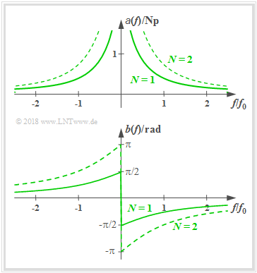
The frequency response of a realizable high–pass (HP) of order $N$ is:
- $$H(f) = \left [\frac{ {\rm j}\cdot f/f_0 }{1 + {\rm j}\cdot f/f_0 }\right ]^N\hspace{0.05cm}.$$
For example the LC high-pass is a first order high-pass. Consequently we can obtain
- the attenuation function:
- $$a(f) =N/2 \cdot \ln [1+( f_0/f)^2] \hspace{0.05cm},$$
- the phase function:
- $$b(f) =-N \cdot \arctan( f_0/f) \hspace{0.05cm},$$
- the attenuation factor for the frequency $f=f_i$:
- $$\alpha_i =|H(f = f_i)| = [1+( f_0/f_i)^2]^{-N/2}$$
- $$\Rightarrow \hspace{0.3cm} x(t)= A_i\cdot \cos(2\pi f_i t) \hspace{0.1cm}\rightarrow \hspace{0.1cm} y(t)= \alpha_i \cdot A_i\cdot \cos(2\pi f_i t)\hspace{0.05cm},$$
- the phase delay for the frequency $f=f_i$:
- $$\tau_i =\frac{b(f_i)}{2\pi f_i} = \frac{-N \cdot \arctan( f_0/f_i)}{2\pi f_i}$$
- $$\Rightarrow \hspace{0.3cm} x(t)= A_i\cdot \cos(2\pi f_i t) \hspace{0.1cm}\rightarrow \hspace{0.1cm} y(t)=A_i\cdot \cos(2\pi f_i (t- \tau_i))\hspace{0.05cm}.$$
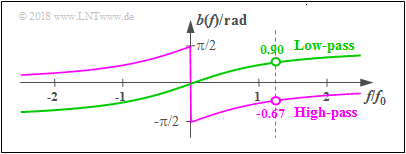
$\text{Example:}$ This graphic shows the phase function $b(f)$ with the cutoff frequency $f_0 = 1\ \rm kHz$ and order $N=1$
- of a low–pass (green curve),
- of a high–pass (violet curve).
The input signal is sinusoidal with frequency $f_{\rm S} = 1.25\ {\rm kHz}$ whereby this signal is only turned on at $t=0$:
- $$x(t) = \left\{ \begin{array}{l} \hspace{0.75cm}0 \\ \sin(2\pi \cdot f_{\rm S} \cdot t ) \\ \end{array} \right.\quad\begin{array}{l} (t < 0), \\ (t>0). \\ \end{array}$$
The left graphic shows the signal $x(t)$. The dashed line marks the first zero at $t = T_0 = 0.8\ {\rm ms}$. The other two graphics show the output signals $y_{\rm LP}(t)$ und $y_{\rm HP}(t)$ of low–pass and high–pass, whereby the change in amplitude was balanced in both cases.
- The first zero of the signal $y_{\rm LP}(t)$ after the low–pass is delayed by $\tau_{\rm LP} = 0.9/(2\pi) \cdot T_0 \approx 0.115 \ {\rm ms}$ compared to the first zero of $x(t)$ ⇒ marked with green arrow, whereby $b_{\rm LP}(f/f_{\rm S} = 0.9 \ {\rm rad})$ was considered.
- In contrast, the phase delay of the high–pass is negative: $\tau_{\rm HP} = -0.67/(2\pi) \cdot T_0 \approx -0.085 \ {\rm ms}$ and therefore the first zero of $y_{\rm HP}(t)$ occurs before the dashed line.
- Following this transient response, in both cases the zero crossings again come in the raster of the period duration $T_0 = 0.8 \ {\rm ms}.$
Remark: The shown signals were created using the interactive applet "Causal systems – Laplace transform".
Attenuation and Phase Distortions
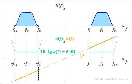
The adjacent figure shows
- the even attenuation function $a(f)$ ⇒ $a(-f) = a(f)$, and
- the uneven function curve $b(f)$ ⇒ $b(-f) = -b(- f)$
of a non–distorting channel. One can see:
- In a distortion–free system the attenuation function $a(f)$ must be constant between$f_{\rm U}$ and $f_{\rm O}$ around the carrier frequency $f_{\rm T}$, where the input signal exists ⇒ $X(f) \ne 0$.
- From the specified constant attenuation value $6 \ \rm dB$ follows for the amplitude response $|H(f)| = 0.5$ ⇒ the signal values of all frequencies are thus halved by the system ⇒ no attenuation distortions.
- In addition, in such a system, the phase function $b(f)$ between $f_{\rm U}$ and $f_{\rm O}$ must increase linearly with the frequency. As a result, all frequency components are delayed by the same phase delay $τ$ ⇒ no phase distortion.
- The delay $τ$ is fixed by the slope of $b(f)$. The phase function $b(f) \equiv 0$ would result in a delay–less system ⇒ $τ = 0$.
The following summary considers that – in this applet – the input signal is always the sum of two harmonic oscillations,
- $$x(t) = x_1(t) + x_2(t) = A_1\cdot \cos\left(2\pi f_1\cdot t- \varphi_1\right)+A_2\cdot \cos\left(2\pi f_2\cdot t- \varphi_2\right), $$
and therefore the channel influence is fully described by the attenuation factors $\alpha_1$ and $\alpha_2$ as well as the phase delays $\tau_1$ and $\tau_2$:
- $$y(t) = \alpha_1 \cdot x_1(t-\tau_1) + \alpha_2 \cdot x_2(t-\tau_2).$$
$\text{Summary:}$
- A signal $y(t)$ is only distortion–free compared to $x(t)$ if $\alpha_1 = \alpha_2= \alpha$ and $\tau_1 = \tau_2= \tau$ ⇒ $y(t) = \alpha \cdot x(t-\tau)$.
- Attenuation distortions occur when $\alpha_1 \ne \alpha_2$. If $\alpha_1 \ne \alpha_2$ and $\tau_1 = \tau_2$, then there are exclusively attenuation distortions.
- Phase distortions occur when $\tau_1 \ne \tau_2$. If $\tau_1 \ne \tau_2$ and $\alpha_1 = \alpha_2$, then there are exclusively phase distortions.
Exercises
- First choose an exercise number.
- An exercise description is displayed.
- Parameter values are adjusted to the respective exercises.
- Click "Hide solution" to display the solution.
Number "0" is a "Reset" button:
- Sets parameters to initial values (when loading the page).
- Displays a "Reset text" to describe the applet further.
(1) We consider the parameters $A_1 = 0.8\ {\rm V}, \ A_2 = 0.6\ {\rm V}, \ f_1 = 0.5\ {\rm kHz}, \ f_2 = 1.5\ {\rm kHz}, \ \varphi_1 = 90^\circ, \ \varphi_2 = 30^\circ$ for the input signal $x(t)$.
- Calculate the signal's period duration $T_0$ and power $P_x$. Can you read the value for $P_x$ off the applet?
$\hspace{1.0cm}\Rightarrow\hspace{0.3cm}T_0 = \big [\hspace{-0.1cm}\text{ greatest common divisor }(0.5 \ {\rm kHz}, \ 1.5 \ {\rm kHz})\big ]^{-1}\hspace{0.15cm}\underline{ = 2.0 \ {\rm ms}};$
$\hspace{1.85cm} P_x = A_1^2/2 + A_2^2/2 \hspace{0.15cm}\underline{= 0.5 \ {\rm V^2}} = P_\varepsilon\text{, if }\hspace{0.15cm}\underline{k_{\rm M} = 0} \ \Rightarrow \ z(t) \equiv 0$.
(2) Vary $\varphi_2$ between $\pm 180^\circ$ while keeping all other parameters from Exercise (1). How does the value of $T_0$ and $P_x$ change?
$\hspace{1.0cm}\Rightarrow\hspace{0.3cm}\text{No changes:}\hspace{0.2cm}\hspace{0.15cm}\underline{ T_0 = 2.0 \ {\rm ms}; \hspace{0.2cm} P_x = 0.5 \ {\rm V^2}}$.
(3) Vary $f_2$ between $0 \le f_2 \le 10\ {\rm kHz}$ while keeping all other parameters from Exercise (1). How does the value of $P_x$ change?
$\hspace{1.0cm}\Rightarrow\hspace{0.3cm}\text{No changes if }f_2 \ne 0\text{ and } f_2 \ne f_1\text{:}\hspace{0.3cm} \hspace{0.15cm}\underline{P_x = 0.5 \ {\rm V^2}}\text{.} \hspace{0.2cm} T_0 \text{ changes if }f_2\text{is not a multiple of }f_1$.
$\hspace{1.85cm}\text{If }f_2 = 0\text{:}\hspace{0.2cm} P_x = A_1^2/2 + A_2^2\hspace{0.15cm}\underline{ = 0.68 \ {\rm V^2}}$. $\hspace{3cm}$
$\hspace{1.85cm}\text{If }f_2 = f_1\text{:}\hspace{0.2cm} P_x = [A_1\cos(\varphi_1) + A_2\cos(\varphi_2)]^2/2 + [A_1\sin(\varphi_1) + A_2\sin(\varphi_2)]^2/2 \text{.} $
$\hspace{1.85cm}\text{With } \varphi_1 = 90^\circ, \ \varphi_2 = 30^\circ\text{:}\hspace{0.3cm}\hspace{0.15cm}\underline{ P_x = 0.74 \ {\rm V^2}}\text{.} $
(4) Keeping the previous input signal $x(t)$, set following parameters
- $\alpha_1 = \alpha_2 = 0.5, \ \tau_1 = \tau_2 = 0.5\ {\rm ms}$, $k_{\rm M} = 1 \text{ and } \tau_{\rm M} = 0$ .
- Are there linear distortions? Calculate the received power $P_y$ and the power $P_\varepsilon$ of the differential signal $\varepsilon(t) = z(t) - x(t)$.
$\hspace{1.0cm}\Rightarrow \hspace{0.3cm}\hspace{0.15cm}\underline{ y(t) = 0.5 \cdot x(t- 1\ {\rm ms})}\text{ is only attenuated and delayed, but not distorted.}$
$\hspace{1.85cm}\text{Received power:}\hspace{0.2cm} P_y = (A_1/2)^2/2 + (A_2/2)^2/2\hspace{0.15cm}\underline{ = 0.125 \ {\rm V^2}}\text{. } P_\varepsilon \text{ is significantly larger:} \hspace{0.1cm} \hspace{0.15cm}\underline{P_\varepsilon = 0.625 \ {\rm V^2}}.$
(5) With the same settings as in Exercise (4), vary the matching parameters $k_{\rm M} \text{ and } \tau_{\rm M}$. How big is the distortion power $P_{\rm D}$?
$\hspace{1.0cm}\Rightarrow \hspace{0.3cm} P_{\rm D}\text{ is equal to }P_\varepsilon \text{ when using the ideal matching parameters:} \hspace{0.2cm}k_{\rm M} = 2 \text{ and } \tau_{\rm M}=T_0 - 0.5\ {\rm ms} = 1.5\ {\rm ms}$
$\hspace{1.0cm}\Rightarrow \hspace{0.3cm}z(t) = x(t)\hspace{0.3cm}\Rightarrow \hspace{0.3cm}\varepsilon(t) = 0\hspace{0.3cm}\Rightarrow \hspace{0.3cm}P_{\rm D}\hspace{0.15cm}\underline{ = P_\varepsilon = 0} \hspace{0.3cm}\Rightarrow \hspace{0.3cm}\text{Neither attenuation nor phase distortion.}$
(6) The channel parameters are now set to: $\alpha_1 = 0.5, \hspace{0.15cm}\underline{\alpha_2 = 0.2}, \ \tau_1 = \tau_2 = 0.5\ {\rm ms}$. Calculate the distortion power $P_{\rm D}$ and the Signal-to-Distortion ratio $(\rm SDR) \ \rho_{\rm D}$.
$\hspace{1.0cm}\Rightarrow \hspace{0.3cm} P_{\rm D} = P_\varepsilon \text{ when using the best matching parameters:} \hspace{0.2cm}\hspace{0.15cm}\underline{k_{\rm M} = 2.24} \text{ and } \hspace{0.15cm}\underline{\tau_{\rm M} = 1.5\ {\rm ms} }\text{:} \hspace{0.2cm}\hspace{0.15cm}\underline{P_{\rm D} = 0.059 \ {\rm V^2}}$.
$\hspace{1.85cm}\text{Attenuation distortions only.} \hspace{0.3cm}\text{Signal-to-Distortion-Ratio}\ \hspace{0.15cm}\underline{\rho_{\rm D} = P_x/P_\varepsilon \approx 8.5}$.
(7) The channel parameters are now set to: $\alpha_1 = \alpha_2 = 0.5, \ \tau_1 \hspace{0.15cm}\underline{= 2\ {\rm ms} }, \ \tau_2 = 0.5\ {\rm ms}$. Calculate the distortion power $P_{\rm D}$ and the the Signal-to-Distortion ratio $\rho_{\rm D}$.
$\hspace{1.0cm}\Rightarrow \hspace{0.3cm} P_{\rm D} = P_\varepsilon \text{when using the best matching parameters:} \hspace{0.2cm}\hspace{0.15cm}\underline{k_{\rm M} = 1.84} \text{ and } \tau_{\rm M}\hspace{0.15cm}\underline{ = 0.15\ {\rm ms} }\text{:} \hspace{0.2cm}\hspace{0.15cm}\underline{P_{\rm D} = 0.071 \ {\rm V^2}}$.
$\hspace{1.85cm}\text{Phase distortions only.} \hspace{0.3cm}\text{Signal-to-Distortion-Ratio}\ \hspace{0.15cm}\underline{\rho_{\rm D} = P_x/P_\varepsilon \approx 7}$.
(8) The channel parameters are now set to: $\hspace{0.15cm}\underline{\alpha_1 = 0.5} , \hspace{0.15cm}\underline{\alpha_2 = 0.2} , \ \hspace{0.15cm}\underline{\tau_1= 0.5\ {\rm ms} }, \ \hspace{0.15cm}\underline{\tau_2 = 0.3\ {\rm ms} }$. Are there attenuation distortions? Are there phase distortions? How can $y(t)$ be approximated? Hint: $\cos(3x) = 4 \cdot \cos^3(x) - 3\cdot \cos(x).$
$\hspace{1.0cm}\Rightarrow\hspace{0.3cm} \text{Both attenuation and phase distortions, because }\alpha_1 \ne \alpha_2\text{ and }\tau_1 \ne \tau_2$.
$\hspace{1.85cm}y(t) = y_1(t) + y_2(t)\ \Rightarrow \ y_1(t) = A_1 \cdot \alpha_1 \cdot \sin[2\pi f_1\ (t- 0.5\ \rm ms)] = -0.4 \ {\rm V} \cdot \cos(2\pi f_1 t)$
$\hspace{1.85cm} y_2(t) = \alpha_2 \cdot x_2(t- \tau_2) \text{ mit }x_2(t) = A_2 \cdot \cos[2\pi f_2\ (t- 30^\circ)] \approx A_2 \cdot \cos[2\pi f_2\ (t- 1/36 \ \rm ms)]$
$\hspace{1.85cm} \Rightarrow \ y_2(t) = 0.12 \ {\rm V} \cdot \cos[2\pi f_2\ (t- 0.328 \ {\rm ms})] \approx -0.12 \ { \rm V} \cdot \cos[2\pi f_2t] $.
$\hspace{1.85cm} \Rightarrow \ y(t) = y_1(t) + y_2(t) \approx -0.4 \ {\rm V} \cdot [\cos(2\pi \cdot f_1\cdot t) + 1/3 \cdot \cos(2\pi \cdot 3 f_1 \cdot t) = -0.533 \ {\rm V} \cdot \cos^3(2\pi f_1 t)$.
(9) Using the parameters from Exercise (8), calculate the distortion power $P_{\rm D}$ and the the Signal-to-Distortion ratio $\rho_{\rm D}$.
$\hspace{1.0cm}\text{Best possible adaptation:} \hspace{0.2cm}\hspace{0.15cm}\underline{k_{\rm M} = 1.96} \text{, } \hspace{0.15cm}\underline{\tau_{\rm M} = 1.65\ {\rm ms} }\text{:} \hspace{0.2cm}\hspace{0.15cm}\underline{P_{\rm D} = 0.15 \ {\rm V^2} },\hspace{0.1cm}\hspace{0.15cm}\underline{\rho_{\rm D} = 0.500/0.15 \approx 3.3}$.
(10) Now we set $A_2 = 0$ and $A_1 = 1\ {\rm V}, \ f_1 = 1\ {\rm kHz}, \ \varphi_1 = 0^\circ$. The channel is a Low-pass of order 1 $\underline{(f_0 = 1\ {\rm kHz})}$.
Are there any attenuation and/or phase distortions? Calculate the channel coefficients $\alpha_1$ and $\tau_1$.
$\hspace{1.0cm}\text{At only one frequency there are neither attenuation nor phase distortions.}$
$\hspace{1.0cm}\text{Attenuation factor for }f_1=f_0\text{ and }N=1\text{: }\alpha_1 =|H(f = f_1)| = [1+( f_1/f_0)^2]^{-N/2} = 2^{-1/2}= 1/\sqrt{2}\hspace{0.15cm}\underline{=0.707},$
$\hspace{1.0cm}\text{Phase factor for }f_1=f_0\text{ and }N=1\text{: }\tau_1 = N \cdot \arctan( f_1/f_0)/(2 \pi f_1)=\arctan( 1)/(2 \pi f_1) =1/(8f_1) \hspace{0.15cm}\underline{=0.125 \ \rm ms}.$
(11) How do the channel parameters change when using a Low-pass of order 2 compared to a Low-pass of order 1 $(f_0 = 1\ {\rm kHz})$?
$\hspace{1.0cm}\alpha_1 = 0.707^2 = 0.5$ and $\tau_1 = 2 \cdot 0.125 = 0.25 \ {\rm ms}$.
$\hspace{1.0cm}\text{The signal }y(t)\text{ is only half as big as }x(t)\text{ and is retarded: The cosine turns into a sine function}$.
(12) What differences arise when using a High-pass of order 2 compared to a Low-pass of order 2 $(f_0 = 1\ {\rm kHz})$?
$\hspace{1.0cm}\text{Since }f_1 = f_0\text{ the attenuation factor }\alpha_1 = 0.5\text{ stays the same and }\tau_1 = -0.25 \ {\rm ms}\text{ which means:}$
$\hspace{1.0cm}\text{The signal }y(t)\text{ is also only half as big as }x(t)\text{ and precedes it: The cosine turns into the Minus–sine function}$.
(13) What differences at the signal $y(t)$ can be observed between the Low-pass and the High-pass of order 2 $(f_0 = 1\ {\rm kHz})$ when you start with the initial input signal according to Exercise (1) and continuously raise $f_2$ up to $10 \ \rm kHz$ ?
$\hspace{1.0cm}\text{With the Low-pass the second term is increasingly suppressed. For }f_2 = 10 \ {\rm kHz}\text{: }y_{\rm LP}(t) \approx 0.8 \cdot x_1(t-0.3 \ \rm ms).$
$\hspace{1.0cm}\text{With the High-pass however the second term dominates. For }f_2 = 10 \ {\rm kHz}\text{: }y_{\rm HP}(t) \approx 0.2 \cdot x_1(t+0.7 \ {\rm ms}) + x_2(t).$
Applet Manual
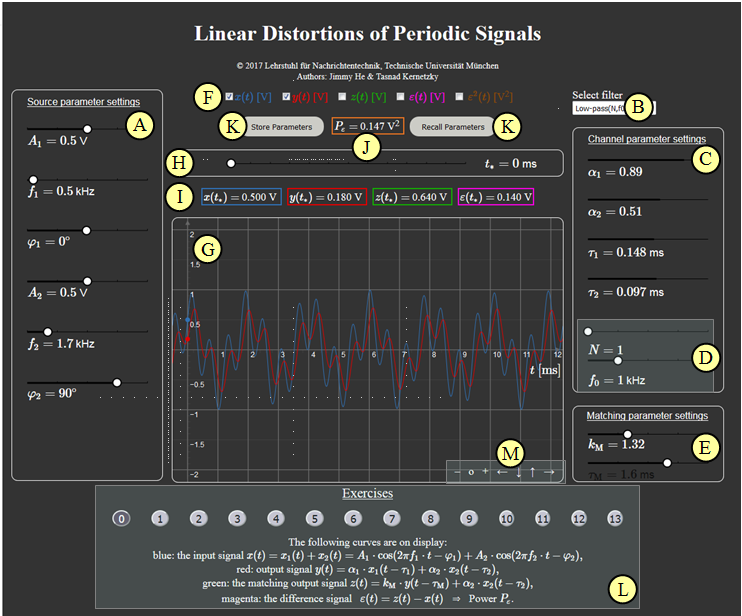
(A) Parameter selection for input signal $x(t)$ per slider: Amplitude, frequency, phase values
(B) Preselection for channel parameters per slider: Low-pass or High-pass
(C) Selction of channel parameters per slider: Dämpfungsfaktoren und Phasenlaufzeiten
(D) Selection of channel parameters for High and Low pass: Order$n$, cutoff frequency $f_0$
(E) Selection of matching parameters $k_{\rm M}$ and $\varphi_{\rm M}$
(F) Selection of the signals to be displayed: $x(t)$, $y(t)$, $z(t)$, $\varepsilon(t)$, $\varepsilon^2(t)$
(G) Graphic display of the signals
(H) Enter the time $t_*$ for the numeric output
( I ) numeric output of the signal values $x(t_*)$, $y(t_*)$, $z(t_*)$ and $\varepsilon(t_*)$
(J) Numeric output of the main result $P_\varepsilon$
(K) Save and reall parameters
(L) Exercises: Exercise selection, description and solution
(M) Variation possibilities for the graphic display
$\hspace{1.5cm}$Zoom–functions "$+$" (scale up), "$-$" (scale down) und $\rm o$ (reset)
$\hspace{1.5cm}$Move with "$\leftarrow$" (section to the left, ordinate to the right), "$\uparrow$" "$\downarrow$" und "$\rightarrow$"
$\hspace{1.5cm}$'Other options:
$\hspace{1.5cm}$Hold shift and scroll: Zoom in on/out of coordinate system,
$\hspace{1.5cm}$Hold shift and left click: Move the coordinate system.
About the Authors
This interactive calculation was designed and realized at the Lehrstuhl für Nachrichtentechnik of the Technische Universität München.
- The original version was created in 2005 by Bettina Hirner as part of her Diploma thesis using "FlashMX–Actionscript" (Supervisor: Günter Söder ).
- In 2018 this Applet was redesigned and updated to "HTML5" by Jimmy He as part of his Bachelor's thesis (Supervisor: Tasnád Kernetzky) .
Once again: Open Applet in new Tab
Open Applet in new Tab English Applet with German WIKI description
