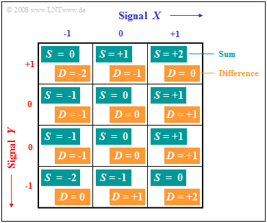
[[File:P_ID146__Sto_Z1_1.png|right|framed|Sum $S$ of two <br>ternary signals $X$ and $Y$]]
Gegeben seien zwei dreistufige Nachrichtenquellen $X$ und $Y$, deren Ausgangssignale jeweils nur die Werte $-1$, $0$ und $+1$ annehmen können. Die Signalquellen sind statistisch voneinander unabhängig.
Let two three-stage message sources $X$ and $Y$ be given, whose output signals can only assume the values $-1$, $0$ and $+1$ respectively. The signal sources are statistically independent of each other.
*Eine einfache Schaltung bildet nun das Summensignal $S = X + Y$.
*A simple circuit now forms the sum signal $S = X + Y$.
*Bei der Signalquelle $X$ treten die Werte $-1$, $0$ und $+1$ mit gleicher Wahrscheinlichkeit auf.
*At the signal source $X$, the values $-1$, $0$ and $+1$ occur with equal probability.
*Bei der Quelle $Y$ ist der Signalwert $0$ doppelt so wahrscheinlich wie die beiden anderen Werte $-1$ bzw. $+1$.
*For source $Y$, the signal value $0$ is twice as likely as the other two values $-1$ and $+1$, respectively.
Hints:
*The exercise belongs to the chapter [[Theory_of_Stochastic_Signals/Einige_grundlegende_Definitionen | Some basic definitions of probability theory]].
''Hinweise:''
*Die Aufgabe gehört zum Kapitel [[Theory_of_Stochastic_Signals/Einige_grundlegende_Definitionen | Einige grundlegende Definitionen der Wahrscheinlichkeitsrechnung]].
*Lösen Sie die Teilaufgaben '''(3)''' und '''(4)''' nach der klassischen Definition.
*Solve the subtasks '''(3)''' and '''(4)''' according to the classical definition.
*Berücksichtigen Sie trotzdem die unterschiedlichen Auftrittshäufigkeiten des Signals $Y$.
*Nevertheless, consider the different occurrence frequencies of the signal $Y$.
*Der Inhalt dieses Abschnitts ist im Lernvideo [[Klassische_Definition_der_Wahrscheinlickeit_(Lernvideo)|Klassische Definition der Wahrscheinlichkeit]] zusammengefasst.
*The topic of this section is illustrated with examples in the (German language) learning video <br>[[Klassische_Definition_der_Wahrscheinlickeit_(Lernvideo)|Klassische Definition der Wahrscheinlichkeit]] $\Rightarrow$ "Classical definition of probability".
Line 26:
Line 23:
===Fragebogen===
===Questions===
<quiz display=simple>
<quiz display=simple>
{Wie groß sind die Auftrittswahrscheinlichkeiten der Signalwerte von $Y$? Wie groß ist die Wahrscheinlichkeit, dass $Y = 0$ ist ?
{What are the probabilities of occurrence of the signal values of $Y$? What is the probability that $Y = 0$ ?
|type="{}"}
|type="{}"}
${\rm Pr}(Y=0) \ = \ $ { 0.5 3% }
${\rm Pr}(Y=0) \ = \ $ { 0.5 3% }
{Wieviele unterschiedliche Signalwerte $(I)$ kann das Summensignal $S$ annehmen? Welche sind dies?
{How many different signal values $(I)$ can the sum signal $S$ assume? Which are these?
|type="{}"}
|type="{}"}
$ I \ = \ $ { 5 3% }
$ I \ = \ $ { 5 3% }
{Mit welchen Wahrscheinlichkeiten treten die in der Teilaufgabe '''(2)''' ermittelten Werte auf? Wie wahrscheinlich ist der Maximalwert $S_{\rm max}$?
{What are the probabilities of the values determined in subtask '''(2)'''? How probable is the maximum value $S_{\rm max}$?
{Wie ändern sich die Wahrscheinlichkeiten, wenn nun anstelle der Summe die Differenz $D = X - Y$ betrachtet wird? Begründen Sie Ihre Antwort.
{How do the probabilities change, if now instead of the sum the difference $D = X - Y$ is considered? Give reasons for your answer.
|type="[]"}
|type="[]"}
+ Die Wahrscheinlichkeiten bleiben gleich.
+ The probabilities remain the same.
- Die Wahrscheinlichkeiten ändern sich. Wie ändern sie sich?
- The probabilities change. How do they change?
Line 53:
Line 50:
</quiz>
</quiz>
===Musterlösung===
===Solution===
{{ML-Kopf}}
{{ML-Kopf}}
'''(1)''' Da die Wahrscheinlichkeiten von $ \pm 1$ gleich sind und ${\rm Pr}(Y = 0) = 2 \cdot {\rm Pr}(Y = 1)$ gilt, erhält man:
'''(1)''' Since the probabilities of $ \pm 1$ are the same and ${\rm Pr}(Y = 0) = 2 \cdot {\rm Pr}(Y = 1)$ holds, we get:
[[File:EN_Sto_Z1_1_c_neu.png|right|frame|400px|Sum and difference of ternary random variables]]
'''(2)''' $S$ can take a total of $\underline {I =5}$ values, namely $0$, $\pm 1$ and $\pm 2$.
[[File:EN_Sto_Z1_1_c.png|right|frame|400px|Summe und Differenz ternärer Zufallsgrößen]]
'''(3)''' Since $Y$ is not equally distributed, one cannot (actually) apply the "Classical Definition of Probability" here.
'''(3)''' Da $Y$ nicht gleichverteilt ist, kann man hier (eigentlich) die "Klassische Definition der Wahrscheinlichkeit" nicht anwenden.
*Teilt man $Y$ jedoch gemäß der Grafik in vier Bereiche auf, wobei man zwei der Bereiche dem Ereignis $Y = 0$ zuordnet, so kann man trotzdem gemäß der klassischen Definition vorgehen.
*However, if we divide $Y$ into four ranges according to the graph, assigning two of the ranges to the event $Y = 0$, we can still proceed according to the classical definition.
*Man erhält dann:
*One then obtains:
:$${\rm Pr}(S = 0) = {4}/{12} = {1}/{3},$$
:$${\rm Pr}(S = 0) = {4}/{12} = {1}/{3},$$
Line 75:
Line 72:
'''(4)''' Aus der Grafik ist auch ersichtlich, dass das Differenzsignal $D$ und das Summensignal $S$ die gleichen Werte mit gleichen Wahrscheinlichkeiten annehmen.
'''(4)''' It is also evident from the graph that the difference signal $D$ and the sum signal $S$ take the same values with equal probabilities.
*Dies war zu erwarten, da ${\rm Pr}(Y = +1) ={\rm Pr}(Y = -1)$ vorgegeben ist ⇒ <u>Lösungsvorschlag 1</u>.
*This was to be expected, since ${\rm Pr}(Y = +1) ={\rm Pr}(Y = -1)$ is given ⇒ <u>Proposed solution 1</u>.
{{ML-Fuß}}
{{ML-Fuß}}
[[Category:Theory of Stochastic Signals: Exercises|^1.1 Einige grundlegende Definitionen
[[Category:Theory of Stochastic Signals: Exercises|^1.1 Some Basic Definitions
Let two three-stage message sources $X$ and $Y$ be given, whose output signals can only assume the values $-1$, $0$ and $+1$ respectively. The signal sources are statistically independent of each other.
A simple circuit now forms the sum signal $S = X + Y$.
At the signal source $X$, the values $-1$, $0$ and $+1$ occur with equal probability.
For source $Y$, the signal value $0$ is twice as likely as the other two values $-1$ and $+1$, respectively.
Solve the subtasks (3) and (4) according to the classical definition.
Nevertheless, consider the different occurrence frequencies of the signal $Y$.
The topic of this section is illustrated with examples in the (German language) learning video Klassische Definition der Wahrscheinlichkeit $\Rightarrow$ "Classical definition of probability".
(2) $S$ can take a total of $\underline {I =5}$ values, namely $0$, $\pm 1$ and $\pm 2$.
(3) Since $Y$ is not equally distributed, one cannot (actually) apply the "Classical Definition of Probability" here.
However, if we divide $Y$ into four ranges according to the graph, assigning two of the ranges to the event $Y = 0$, we can still proceed according to the classical definition.