Difference between revisions of "Aufgaben:Exercise 3.3: Moments for Cosine-square PDF"
| (3 intermediate revisions by 2 users not shown) | |||
| Line 29: | Line 29: | ||
<quiz display=simple> | <quiz display=simple> | ||
| − | {Which of the following statements are true for any given PDF $f_x(x)$ ? Used are the following quantities: linear mean $m_1$, | + | {Which of the following statements are true for any given PDF $f_x(x)$ ? Used are the following quantities: linear mean $m_1$, second moment $m_2$, variance $\sigma^2$. |
|type="[]"} | |type="[]"} | ||
- $m_2 = 0$, if $m_1 \ne 0$. | - $m_2 = 0$, if $m_1 \ne 0$. | ||
| Line 44: | Line 44: | ||
| − | {What is the | + | {What is the standard deviation of the signal $x(t)$? |
|type="{}"} | |type="{}"} | ||
$\sigma_x \ = \ $ { 0.722 3% } | $\sigma_x \ = \ $ { 0.722 3% } | ||
| Line 61: | Line 61: | ||
| − | {What is the | + | {What is the standard deviation of the signal $y(t)$? |
|type="{}"} | |type="{}"} | ||
$\sigma_y\ = \ $ { 0.361 3% } | $\sigma_y\ = \ $ { 0.361 3% } | ||
| Line 84: | Line 84: | ||
| − | '''(3)''' The standard deviation of the signal $x(t)$ is equal to the | + | '''(3)''' The standard deviation of the signal $x(t)$ is equal to the standard deviation $\sigma_x$ or equal to the root of the variance $\sigma_x^2$. |
| − | *Since the random variable $x$ has mean $m_x {= 0}$, the variance is equal to the | + | *Since the random variable $x$ has mean $m_x {= 0}$, the variance is equal to the second moment according to Steiner's theorem. |
*This is also referred to as the power $($with respect to $1 \ \rm \Omega)$ in the context of signals. Thus: | *This is also referred to as the power $($with respect to $1 \ \rm \Omega)$ in the context of signals. Thus: | ||
:$$\sigma_x^{\rm 2}=\int_{-\infty}^{+\infty}x^{\rm 2}\cdot f_x(x)\hspace{0.1cm}{\rm d}x=2 \cdot \int_{\rm 0}^{\rm 2} x^2/2 \cdot \cos^2({\pi}/4\cdot\it x)\hspace{0.1cm} {\rm d}x.$$ | :$$\sigma_x^{\rm 2}=\int_{-\infty}^{+\infty}x^{\rm 2}\cdot f_x(x)\hspace{0.1cm}{\rm d}x=2 \cdot \int_{\rm 0}^{\rm 2} x^2/2 \cdot \cos^2({\pi}/4\cdot\it x)\hspace{0.1cm} {\rm d}x.$$ | ||
| Line 107: | Line 107: | ||
'''(6)''' The mean value does not change the variance and rms. | '''(6)''' The mean value does not change the variance and rms. | ||
| − | *By compressing by the factor $2$ the | + | *By compressing by the factor $2$ the standard deviation becomes smaller compared to subtask '''(3)''' also by this factor: |
:$$\sigma_y=\sigma_x/\rm 2\hspace{0.15cm}\underline{\approx 0.361}.$$ | :$$\sigma_y=\sigma_x/\rm 2\hspace{0.15cm}\underline{\approx 0.361}.$$ | ||
{{ML-Fuß}} | {{ML-Fuß}} | ||
Latest revision as of 14:20, 18 January 2023
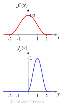
As in Exercise 3.1 and Exercise 3. 2 we consider the random variable restricted to the range of values from $-2$ to $+2$ with the following PDF in this section:
- $$f_x(x)= {1}/{2}\cdot \cos^2({\pi}/{4}\cdot { x}).$$
Next to this, we consider a second random variable $y$ that returns only values between $0$ and $2$ with the following PDF:
- $$f_y(y)=\sin^2({\pi}/{2}\cdot y).$$
- Both probability density functions are shown in the graph.
- Outside the ranges $-2 < x < +2$ resp. $0 < x < +2$, the followings holds: $f_x(x) = 0$ resp. $f_y(y) = 0$.
- Both random variables can be taken as (normalized) instantaneous values of the associated random signals $x(t)$ or $y(t)$ resp.
Hints:
- This exercise belongs to the chapter Expected values and moments.
- To solve this problem, you can use the following indefinite integral:
- $$\int x^{2}\cdot {\cos}(ax)\,{\rm d}x=\frac{2 x}{ a^{ 2}}\cdot \cos(ax)+ \left [\frac{x^{\rm 2}}{\it a} - \frac{\rm 2}{\it a^{\rm 3}} \right ]\cdot \rm sin(\it ax \rm ) .$$
Questions
Solution
- The first statement is never true, as is evident from the "Steiner's theorem".
- The second statement is only valid in the (trivial) special case $x = 0$.
However, there are also zero-mean random variables with asymmetric PDF.
- This means: Statement 6 is not always true.
(2) Because of the PDF symmetry with respect to $x = 0$ it follows that for the linear mean $m_x \hspace{0.15cm}\underline{= 0}$.
(3) The standard deviation of the signal $x(t)$ is equal to the standard deviation $\sigma_x$ or equal to the root of the variance $\sigma_x^2$.
- Since the random variable $x$ has mean $m_x {= 0}$, the variance is equal to the second moment according to Steiner's theorem.
- This is also referred to as the power $($with respect to $1 \ \rm \Omega)$ in the context of signals. Thus:
- $$\sigma_x^{\rm 2}=\int_{-\infty}^{+\infty}x^{\rm 2}\cdot f_x(x)\hspace{0.1cm}{\rm d}x=2 \cdot \int_{\rm 0}^{\rm 2} x^2/2 \cdot \cos^2({\pi}/4\cdot\it x)\hspace{0.1cm} {\rm d}x.$$
- With the relation $\cos^2(\alpha) = 0.5 \cdot \big[1 + \cos(2\alpha)\big]$ it follows:
- $$\sigma_x^2=\int_{\rm 0}^{\rm 2}{x^{\rm 2}}/{\rm 2} \hspace{0.1cm}{\rm d}x + \int_{\rm 0}^{\rm 2}{x^{\rm 2}}/{2}\cdot \cos({\pi}/{\rm 2}\cdot\it x) \hspace{0.1cm} {\rm d}x.$$
- These two standard integrals can be found in tables. One obtains with $a = \pi/2$:
- $$\sigma_x^{\rm 2}=\left[\frac{x^{\rm 3}}{\rm 6} + \frac{x}{a^2}\cdot {\cos}(a x) + \left( \frac{x^{\rm2}}{{\rm2}a} - \frac{1}{a^3} \right) \cdot \sin(a \cdot x)\right]_{x=0}^{x=2} \hspace{0.5cm} \rightarrow \hspace{0.5cm} \sigma_{x}^{\rm 2}=\frac{\rm 4}{\rm 3}-\frac{\rm 8}{\rm \pi^2}\approx 0.524\hspace{0.5cm} \Rightarrow \hspace{0.5cm}\sigma_x \hspace{0.15cm}\underline{\approx 0.722}.$$
(4) Correct is the first mentioned suggestion:
- The variant $y = 2x$ would yield a random variable distributed between $-4$ and $+4$.
- In the last proposition $y = x/2-1$ the mean would be $m_y = -1$.
(5) From the graph on the specification sheet it is already obvious that $m_y \hspace{0.15cm}\underline{=+1}$ must hold.
(6) The mean value does not change the variance and rms.
- By compressing by the factor $2$ the standard deviation becomes smaller compared to subtask (3) also by this factor:
- $$\sigma_y=\sigma_x/\rm 2\hspace{0.15cm}\underline{\approx 0.361}.$$
