Difference between revisions of "Aufgaben:Exercise 3.6: Noisy DC Signal"
From LNTwww
m (Text replacement - "rms value" to "standard deviation") |
|||
| Line 34: | Line 34: | ||
| − | {Calculate the standard deviation | + | {Calculate the standard deviation of the signal $x(t)$. |
|type="{}"} | |type="{}"} | ||
$\sigma_x \ = \ $ { 1 3% } $\ \rm V$ | $\sigma_x \ = \ $ { 1 3% } $\ \rm V$ | ||
| Line 68: | Line 68: | ||
:$$\sigma_{x}^{\rm 2}=m_{\rm 2 \it x}-m_{x}^{\rm 2}. $$ | :$$\sigma_{x}^{\rm 2}=m_{\rm 2 \it x}-m_{x}^{\rm 2}. $$ | ||
| − | *The | + | *The second order moment $m_{2x}$ is equal to the $($referred to $1\hspace{0.05cm} \Omega)$ total power $P_x = 5\hspace{0.05cm}\rm V^2$. |
*With the mean $m_x = 2\hspace{0.05cm}\rm V$ it follows for the standard deviation: | *With the mean $m_x = 2\hspace{0.05cm}\rm V$ it follows for the standard deviation: | ||
:$$\sigma_{x} = \sqrt{5\hspace{0.05cm}\rm V^2 - (2\hspace{0.05cm}\rm V)^2} \hspace{0.15cm}\underline{= 1\hspace{0.05cm}\rm V}.$$ | :$$\sigma_{x} = \sqrt{5\hspace{0.05cm}\rm V^2 - (2\hspace{0.05cm}\rm V)^2} \hspace{0.15cm}\underline{= 1\hspace{0.05cm}\rm V}.$$ | ||
| Line 74: | Line 74: | ||
| − | '''(3)''' The CDF of a Gaussian random variable $($mean $m_x$, | + | '''(3)''' The CDF of a Gaussian random variable $($mean $m_x$, standard deviation $\sigma_x)$ is with the Gaussian error integral: |
:$$F_x(r)=\rm\phi(\it\frac{r-m_x}{\sigma_x}\rm ).$$ | :$$F_x(r)=\rm\phi(\it\frac{r-m_x}{\sigma_x}\rm ).$$ | ||
Latest revision as of 17:02, 17 February 2022
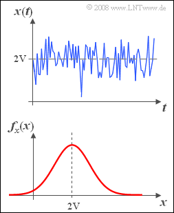
A DC signal $s(t) = 2\hspace{0.05cm}\rm V$ is additively overlaid by a noise signal $n(t)$.
- In the upper picture you can see a section of the sum signal $x(t)=s(t)+n(t).$
- The probability density function $\rm (PDF)$ of the signal $x(t)$ is shown below.
- The $($related to the resistor $1\hspace{0.05cm} \Omega)$ total power of this signal is $P_x = 5\hspace{0.05cm}\rm V^2$.
Hints:
- The exercise belongs to the chapter Gaussian Distributed Random Variables.
- Use the complementary Gaussian error integral ${\rm Q}(x)$ to solve.
- The following are some values of this monotonically decreasing function:
- $$\rm Q(0) = 0.5,\hspace{0.5cm} Q(1) = 0.1587, \hspace{0.5cm}\rm Q(2) = 0.0227, \hspace{0.5cm} Q(3) = 0.0013. $$
Questions
Solution
(1) Correct are solutions 2 and 4:
- The uniform signal $s(t)$ is not uniformly distributed, rather its PDF consists of only one Dirac delta function at $m_x = 2\hspace{0.05cm}\rm V$ with weight $1$.
- The signal $n(t)$ is Gaussian and mean-free ⇒ $m_n = 0$.
- Therefore the sum signal $x(t)$ is also Gaussian, but now with mean $m_x = 2\hspace{0.05cm}\rm V$.
- This is due to the DC signal alone $s(t) = 2\hspace{0.05cm}\rm V$.
(2) According to Steiner's theorem:
- $$\sigma_{x}^{\rm 2}=m_{\rm 2 \it x}-m_{x}^{\rm 2}. $$
- The second order moment $m_{2x}$ is equal to the $($referred to $1\hspace{0.05cm} \Omega)$ total power $P_x = 5\hspace{0.05cm}\rm V^2$.
- With the mean $m_x = 2\hspace{0.05cm}\rm V$ it follows for the standard deviation:
- $$\sigma_{x} = \sqrt{5\hspace{0.05cm}\rm V^2 - (2\hspace{0.05cm}\rm V)^2} \hspace{0.15cm}\underline{= 1\hspace{0.05cm}\rm V}.$$
(3) The CDF of a Gaussian random variable $($mean $m_x$, standard deviation $\sigma_x)$ is with the Gaussian error integral:
- $$F_x(r)=\rm\phi(\it\frac{r-m_x}{\sigma_x}\rm ).$$
- The cumulative distribution function at the point $r = 0\hspace{0.05cm}\rm V$ is equal to the probability that $x$ is less than or equal to $0\hspace{0.05cm}\rm V$ .
- But for continuous random variables, ${\rm Pr}(x \le r) = {\rm Pr}(x < r)$ also holds .
- Using the complementary Gaussian error integral, we obtain:
- $$\rm Pr(\it x < \rm 0\,V)=\rm \phi(\rm \frac{-2\,V}{1\,V})=\rm Q(\rm 2)\hspace{0.15cm}\underline{=\rm 2.27\%}.$$
(4) Because of the symmetry around the mean $m_x = 2\hspace{0.05cm}\rm V$ this gives the same probability, viz.
- $$\rm Pr(\it x > \rm 4\,V)\hspace{0.15cm}\underline{=\rm 2.27\%}.$$
(5) The probability that $x$ is greater than $3\hspace{0.05cm}\rm V$ is given by.
- $${\rm Pr}( x > 3\text{ V}) = 1- F_x(\frac{3\text{ V}-2\text{ V}}{1\text{ V}})=\rm Q(\rm 1)=\rm 0.1587.$$
- For the sought probability one obtains from it:
- $$\rm Pr(3\,V\le \it x \le \rm 4\,V)= \rm Pr(\it x > \rm 3\,V)- \rm Pr(\it x > \rm 4\,V) = 0.1587 - 0.0227\hspace{0.15cm}\underline{=\rm 13.6\%}. $$
