We consider a 2D–random variable $(x, y)$ whose components arise respectively as linear combinations of two random variables $u$ and $v$ :
We consider a two-dimensional random variable $(x,\hspace{0.08cm} y)$ whose components arise as linear combinations of two random variables $u$ and $v$:
:$$x=2u-2v+1,$$
:$$x=2u-2v+1,$$
:$$y=u+3v.$$
:$$y=u+3v.$$
Further, note:
Further, note:
*The two statistically independent random variables $u$ and $v$ are each equally distributed between $0$ and $1$.
*The two statistically independent random variables $u$ and $v$ are each uniformly distributed between $0$ and $1$.
*In the figure you can see the 2D–PDF. Within the parallelogram drawn in blue holds:
*In the figure you can see the joint PDF. Within the parallelogram drawn in blue holds:
:$$f_{xy}(x, y) = H = {\rm const.}$$
:$$f_{xy}(x,\hspace{0.08cm} y) = H = {\rm const.}$$
*Outside the parallelogram no values are possible: $f_{xy}(x, y) = 0$.
*Outside the parallelogram no values are possible: $f_{xy}(x,\hspace{0.08cm} y) = 0$.
Hints:
*The exercise belongs to the chapter [[Theory_of_Stochastic_Signals/Linear_Combinations_of_Random_Variables|Linear Combinations of Random Variables]].
*Reference is also made to the page [[Theory_of_Stochastic_Signals/Two-Dimensional_Random_Variables#Regression_line|Regression line]].
''Hints:''
*We also refer here to the interactive applet [[Applets:Korrelationskoeffizient_%26_Regressionsgerade|Correlation coefficient and regression line]]
*The exercise belongs to the chapter [[Theory_of_Stochastic_Signals/Linear_Combinations_of_Random_Variables|Linear_Combinations of Random Variables]].
*Assume - if possible - the given equations. Use the information of the above sketch mainly only to check your results.
*Reference is also made to the page [[/Theory_of_Stochastic_Signals/Two-Dimensional_Random_Variables#Regression_line|regression line]].
*We also refer here to the interactive applet [Applets:Korrelationskoeffizient_%26_Regressionsgerade|Correlation coefficient and regression line]]
*Assume - if possible - the given equations Use the information of the above sketch mainly only to check your results.
Line 33:
Line 30:
<quiz display=simple>
<quiz display=simple>
{Wie groß ist die Höhe $H$ der 2D–WDF innerhalb des Parallelogramms?
{What is the height $H$ of the joint PDF within the parallelogram?
|type="{}"}
|type="{}"}
$H \ = \ $ { 0.125 3% }
$H \ = \ $ { 0.125 3% }
{Welche Werte von $u$ und $v$ liegen dem Eckpunkt $(-1, 3)$ zugrunde?
{Berechnen Sie den Korrelationskoeffizienten $\rho_{xy}$.
{Calculate the correlation coefficient $\rho_{xy}$.
|type="{}"}
|type="{}"}
$\rho_{xy}\ = \ $ { -0.457--0.437 }
$\rho_{xy}\ = \ $ { -0.457--0.437 }
{Wie lautet die Korrelationsgerade $y=K(x)$? Bei welchem Punkt $y_0$ schneidet diese die $y$-Achse?
{What is the regression line $\rm (RL)$? At what point $y_0$ does it intersect the $y$–axis?
|type="{}"}
|type="{}"}
$y_0\ = \ $ { 2.5 3% }
$y_0\ = \ $ { 2.5 3% }
{Berechnen Sie die Randwahrscheinlichkeitsdichtefunktion $f_x(x)$. Wie groß ist die Wahrscheinlichkeit, dass die Zufallsgröße $x$ negativ ist?
{Calculate the marginal probability density function $f_x(x)$. What is the probability that the random variable $x$ is negative?
|type="{}"}
|type="{}"}
${\rm Pr}(x < 0)\ = \ $ { 0.125 3% }
${\rm Pr}(x < 0)\ = \ $ { 0.125 3% }
{Berechnen Sie die Randwahrscheinlichkeitsdichtefunktion $f_y(y)$. Wie groß ist die Wahrscheinlichkeit, dass die Zufallsgröße $y >3$ ist?
{Calculate the marginal probability density function $f_y(y)$. What is the probability that the random variablee $y >3$?
|type="{}"}
|type="{}"}
${\rm Pr}(y > 3)\ = \ $ { 0.167 3% }
${\rm Pr}(y > 3)\ = \ $ { 0.167 3% }
Line 66:
Line 63:
</quiz>
</quiz>
===Musterlösung===
===Solution===
{{ML-Kopf}}
{{ML-Kopf}}
'''(1)''' Die Fläche des Parallelogramms kann aus zwei gleich großen Dreiecken zusammengesetzt werden.
'''(1)''' The area of the parallelogram can be composed of two triangles of equal size.
*The area of the triangle $(1,0)\ (1,4)\ (-1,3)$ gives $0.5 · 4 · 2 = 4$.
*Die Gesamtfläche ist doppelt so groß: $F = 8$.
*The total area is double: $F = 8$.
*Da das WDF–Volumen stets $1$ ist, gilt $H= 1/F\hspace{0.15cm}\underline{ = 0.125}$.
*Since the PDF volume is always $1$ , then $H= 1/F\hspace{0.15cm}\underline{ = 0.125}$.
'''(2)''' Der minimale Wert von $x$ ergibt sich für $\underline{ u=0}$ und $\underline{ v=1}$.
'''(2)''' The minimum value of $x$ is obtained for $\underline{ u=0}$ and $\underline{ v=1}$.
*Daraus folgen aus obigen Gleichungen die Ergebnisse $x= -1$ und $y= +3$.
*From the above equations, the results $x= -1$ and $y= +3$ follow.
'''(3)''' Die im Theorieteil angegebene Gleichung gilt allgemein, also für jede beliebige WDF der beiden statistisch unabhängigen Größen $u$ und $v$,
'''(3)''' The equation given in the theory section is valid in general, i.e., for any PDF of the two statistically independent variables $u$ and $v$, as long as they have equal standard deviations $(\sigma_u = \sigma_v)$.
*so lange diese gleiche Streuungen aufweisen $(\sigma_u = \sigma_v)$.
'''(4)''' Die Korrelationsgerade lautet allgemein:
*From the linear means $m_u = m_v = 0.5$ and the equations given in the problem statement, we obtain $m_x = 1$ and $m_y = 2$.
*Aus den linearen Mittelwerten $m_u = m_v = 0.5$ und den in der Aufgabenstellung angegebenen Gleichungen erhält man $m_x = 1$ und $m_y = 2$.
*Daraus folgt der Wert $y_0=K(x=0)\hspace{0.15cm}\underline{ = 2.5}$
*From this follows with $x=0$ the value $y_0=\hspace{0.15cm}\underline{ = 2.5}$
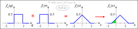
'''(5)''' Mit den Hilfsgrößen $q= 2u$, $r= -2v$ und $s= x-1$ gilt der Zusammenhang: $s= q+r$.
'''(5)''' With the auxiliary quantities $q= 2u$, $r= -2v$ and $s= x-1$: $s= q+r$.
[[File:P_ID414__Sto_A_4_8_e.png|right|frame|Triangular PDF $f_x(x)$]]
*Since $u$ and $v$ are each uniformly distributed between $0$ and $1$, $q$ has a uniform distribution in the range from $0$ to $2$ and $r$ is uniformly distributed between $-2$ and $0$.
*In addition, since $q$ and $r$ are not statistically dependent on each other, the PDF of the sum is:
:$$f_s(s) = f_q(q) \star f_r(r).$$
*The addition $x = s+1$ leads to a shift of the triangular–PDF by $1$ to the right.
*For the sought probability (highlighted in green in the graphic) therefore holds:
*Da $u$ und $v$ jeweils zwischen $0$ und $1$ gleichverteilt sind, besitzt $q$ eine Gleichverteilung im Bereich von $0$ bis $2$ und $r$ ist gleichverteilt zwischen $-2$ und $0$.
*Da zudem $q$ und $r$ nicht statistisch voneinander abhängen, gilt für die WDF der Summe:
We consider a two-dimensional random variable $(x,\hspace{0.08cm} y)$ whose components arise as linear combinations of two random variables $u$ and $v$:
$$x=2u-2v+1,$$
$$y=u+3v.$$
Further, note:
The two statistically independent random variables $u$ and $v$ are each uniformly distributed between $0$ and $1$.
In the figure you can see the joint PDF. Within the parallelogram drawn in blue holds:
$$f_{xy}(x,\hspace{0.08cm} y) = H = {\rm const.}$$
Outside the parallelogram no values are possible: $f_{xy}(x,\hspace{0.08cm} y) = 0$.
(1) The area of the parallelogram can be composed of two triangles of equal size.
The area of the triangle $(1,0)\ (1,4)\ (-1,3)$ gives $0.5 · 4 · 2 = 4$.
The total area is double: $F = 8$.
Since the PDF volume is always $1$ , then $H= 1/F\hspace{0.15cm}\underline{ = 0.125}$.
(2) The minimum value of $x$ is obtained for $\underline{ u=0}$ and $\underline{ v=1}$.
From the above equations, the results $x= -1$ and $y= +3$ follow.
(3) The equation given in the theory section is valid in general, i.e., for any PDF of the two statistically independent variables $u$ and $v$, as long as they have equal standard deviations $(\sigma_u = \sigma_v)$.
With $A = 2$, $B = -2$, $D = 1$ and $E = 3$ we obtain:
From this follows with $x=0$ the value $y_0=\hspace{0.15cm}\underline{ = 2.5}$
(5) With the auxiliary quantities $q= 2u$, $r= -2v$ and $s= x-1$: $s= q+r$.
Triangular PDF $f_x(x)$
Since $u$ and $v$ are each uniformly distributed between $0$ and $1$, $q$ has a uniform distribution in the range from $0$ to $2$ and $r$ is uniformly distributed between $-2$ and $0$.
In addition, since $q$ and $r$ are not statistically dependent on each other, the PDF of the sum is:
$$f_s(s) = f_q(q) \star f_r(r).$$
The addition $x = s+1$ leads to a shift of the triangular–PDF by $1$ to the right.
For the sought probability (highlighted in green in the graphic) therefore holds: