Difference between revisions of "Aufgaben:Exercise 5.6: Error Correlation Duration"
| (One intermediate revision by one other user not shown) | |||
| Line 58: | Line 58: | ||
$\varphi_{e0} \ = \ ${ 0.091 3% } $\ \cdot 10^{-2}$ | $\varphi_{e0} \ = \ ${ 0.091 3% } $\ \cdot 10^{-2}$ | ||
| − | {What result is obtained for the error correlation | + | {What result is obtained for the error correlation duration $D_{\rm K}$ with the quantities $A$ and $B$ defined in front? |
|type="()"} | |type="()"} | ||
- $D_{\rm K} = A \cdot B$, | - $D_{\rm K} = A \cdot B$, | ||
Latest revision as of 14:22, 19 October 2022
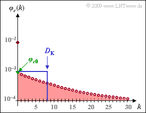
The graph shows the error correlation function (ECF) of the Gilbert–Elliott model with the parameters
- $$p_{\rm G} \hspace{-0.1cm} \ = \ \hspace{-0.1cm} 0.001, \hspace{0.2cm}p_{\rm B} = 0.1,\hspace{0.2cm} {\rm Pr}(\rm G\hspace{0.05cm}|\hspace{0.05cm} B)\hspace{-0.1cm} \ = \ \hspace{-0.1cm} 0.1, \hspace{0.2cm} {\rm Pr}(\rm B\hspace{0.05cm}|\hspace{0.05cm} G) = 0.01\hspace{0.05cm}$$
in logarithmic representation.
This model is discussed in detail in "Exercise 5.6Z". In particular, the error correlation function (ECF) is also calculated in this exercise. With the auxiliary quantities
- $$A \hspace{-0.1cm} \ = \ \hspace{-0.1cm} (p_{\rm B}- p_{\rm M}) \cdot (p_{\rm M}- p_{\rm G})\hspace{0.05cm},$$
- $$B\hspace{-0.1cm} \ = \ \hspace{-0.1cm} {\rm Pr}(\rm B\hspace{0.05cm}|\hspace{0.05cm} G) + {\rm Pr}(\rm G\hspace{0.05cm}|\hspace{0.05cm} B)$$
it can be written for:
- $$\varphi_{e}(k) = \left\{ \begin{array}{c} p_{\rm M} \\ p_{\rm M}^2 + A \cdot (1-B)^k \end{array} \right.\quad \begin{array}{*{1}c} f{\rm or }\hspace{0.15cm}k = 0 \hspace{0.05cm}, \\ f{\rm or }\hspace{0.15cm} k > 0 \hspace{0.05cm}.\\ \end{array}$$
This is a burst error channel. To quantitatively describe the statistical bonds, one often uses the correlation term according to the following definition:
- $$D_{\rm K} = \frac{1}{\varphi_{e0} - p_{\rm M}^2} \cdot \sum_{k = 1 }^{\infty}\hspace{0.1cm}\big [\varphi_{e}(k) - p_{\rm M}^2 \big]\hspace{0.05cm}.$$
The reference value $\varphi_{e0}$ is obtained by extrapolation of the error correlation function to the point $k = 0$. If, as here, the ECF curve is given analytically, $\varphi_{e0}$ can also be calculated by inserting the value $k = 0$ into the equation which is actually only valid for $k > 0$.
Notes:
- The exercise belongs to the chapter "Burst Error Channels".
- Reference is made in particular to the section "Error correlation function of the Gilbert-Elliott model".
Questions
Solution
- From the graph on the information section, one can read $p_{\rm M} \ \underline {= 0.01}$.
- In "Exercise 5.6Z", this value is calculated in a different way.
(2) If we insert the parameter $k = 0$ into the lower ECF equation, which is actually only valid for $k > 0$, we obtain the extrapolation value we are looking for.
- $$\varphi_{e0} \hspace{-0.1cm} \ = \ \hspace{-0.1cm} p_{\rm M}^2 + (p_{\rm B}- p_{\rm M}) \cdot (p_{\rm M}- p_{\rm G})\hspace{0.05cm} = 10^{-4} + (0.1- 0.01) \cdot (0.01- 0.001)=10^{-4} + 0.09 \cdot 0.009 \hspace{0.15cm}\underline {\approx 0.091 \cdot 10^{-2}}\hspace{0.05cm}.$$
(3) According to the general definition equation, the following holds for the error correlation period
- $$D_{\rm K} = \frac{1}{\varphi_{e0} - p_{\rm M}^2} \cdot \sum_{k = 1 }^{\infty}\hspace{0.1cm} [\varphi_{e}(k) - p_{\rm M}^2]\hspace{0.05cm}.$$
- With the expressions
- $$A \hspace{-0.1cm} \ = \ \hspace{-0.1cm} (p_{\rm B}- p_{\rm M}) \cdot (p_{\rm M}- p_{\rm G}) = \varphi_{e0} - p_{\rm M}^2\hspace{0.05cm},$$
- $$B\hspace{-0.1cm} \ = \ \hspace{-0.1cm} {\rm Pr}(\rm B\hspace{0.05cm}|\hspace{0.05cm} G) + {\rm Pr}(\rm G\hspace{0.05cm}|\hspace{0.05cm} B)$$
- this equation can be written as follows:
- $$D_{\rm K} = {1}/{A} \cdot \sum_{k = 1 }^{\infty}\hspace{0.1cm} A \cdot (1 - B)^k = \sum_{k = 1 }^{\infty}\hspace{0.1cm} (1 - B)^k\hspace{0.05cm}.$$
- Using the summation formula of a geometric series, this gives the final result:
- $$D_{\rm K} = {1}/{B} - 1 = \frac{1}{{\rm Pr}(\rm B\hspace{0.05cm}|\hspace{0.05cm} G) + {\rm Pr}(\rm G\hspace{0.05cm}|\hspace{0.05cm} B)} - 1\hspace{0.05cm}.$$
- So solution 3 is correct.
(4) With ${\rm Pr(B|G)} = 0.01$ and ${\rm Pr(G|B)} = 0.1$ we get
- $$D_{\rm K} = \frac{1}{0.01 + 0.1} - 1 \hspace{0.15cm}\underline {\approx 8.091}\hspace{0.05cm}.$$
(5) Only solution 1 is correct, as shown in the sample solutions to the last subtasks:
- Thus the correlation term is fixed, for example:
- With ${\rm Pr(B\hspace{0.05cm}|\hspace{0.05cm}G)} = 0.1$ and $\rm Pr(G\hspace{0.05cm}|\hspace{0.05cm}B) = 0.01$ we get the same $D_{\rm K} = 8.091$ as with $\rm Pr(B\hspace{0.05cm}|\hspace{0.05cm}G) = 0.01$ and $\rm Pr(G\hspace{0.05cm}|\hspace{0.05cm}B) = 0.1$.
- But now the mean error probability $p_{\rm M} \approx 9.1\%$ instead of $1\%$, respectively for $p_{\rm G} = 0.001$ and $p_{\rm B} = 0.1$.
- The last statement is also false. This statement would only be true if $\varphi_e(k)$ was plotted linearly and not logarithmically as here.
