Difference between revisions of "Applets:Principle of 4B3T Coding"
| (13 intermediate revisions by 2 users not shown) | |||
| Line 3: | Line 3: | ||
== Applet Description== | == Applet Description== | ||
<br> | <br> | ||
| − | + | The applet illustrates the principle of $\rm 4B3T$ coding. Here, in each case a block of four binary symbols is replaced by a sequence of three ternary symbols. This results in a relative code redundancy of just under $16\%$, which is used to achieve equal signal freedom. | |
| − | + | The recoding of the sixteen possible binary blocks into the corresponding ternary blocks could in principle be done according to a fixed code table. However, to further improve the spectral characteristics of these codes, the 4B3T codes always use multiple code tables, which are selected block by block according to the "running digital sum" $(\rm RDS)$ . | |
| − | + | In the applet, the corresponding code tables are given in the lower area, alternatively for | |
| − | * | + | * the $\rm MS43$ code (from: $\rm M$onitored $\rm S$um $\rm 4$B$\rm 3$T–code), and |
| − | * | + | * the $\rm MMS43$ code (from: $\rm M$odified $\rm MS43$). |
| − | + | Input parameters are, besides the desired code (MS43 or MMS43), the RDS start value $\rm RDS_0$ and twelve binary source symbols $q_\nu \in \{0,\ 1\}$, either by hand, by default $($source symbol sequence $\rm A$, $\rm B$, $\rm C)$ or by random generator. | |
| − | + | Two different modes are offered by the program: | |
| − | * | + | *In the "Step" mode, the three blocks are processed successively (in each case defining the three ternary symbols, updating the RDS value and thus defining the code table for the next block. |
| − | * | + | *In the "Total" mode, only the coding results are displayed, but simultaneously for the two possible codes and in each case for all four possible RDS ;start values. The graphic and the RDS output block on the right refer to the settings made. |
| Line 24: | Line 24: | ||
==Theoretical Background== | ==Theoretical Background== | ||
| − | === | + | ===Classification of various coding methods === |
<br> | <br> | ||
| − | + | We consider the digital transmission model shown. As can be seen from this block diagram, depending on the target direction, a distinction is made between three different types of coding, each realized by the encoder at the transmitting end and the associated decoder at the receiving end: | |
| − | [[File: | + | [[File:EN_Inf_T_2_1_S1_v2.png|right|frame|Simplified model of a digital transmission system]] |
| − | *$\text{ | + | *$\text{Source coding:}$ Removing (unnecessary) redundancy to store or transmit data as efficiently as possible ⇒ Data compression. Example: Differential pulse code modulation $\rm (DPCM)$ in image coding. |
| − | *$\text{ | + | *$\text{Channel coding:}$ Targeted addition of (meaningful) redundancy, which can be used at the receiver for error detection or error detection. Main representatives: Block codes, convolutional codes, turbo codes. |
| − | *$\text{ | + | *$\text{Line coding:}$ Recoding of source symbols to adapt the signal to the spectral characteristics of the channel and receiving equipment, for example to achieve a transmitted signal free of equal signals $x(t)$ for a channel with $H_{\rm K}(f = 0) = 0$ . |
<br clear=all> | <br clear=all> | ||
| − | + | In the case of line codes, a further distinction is made: | |
| − | *$\text{ | + | *$\text{Symbol-wise coding:}$ With each incoming binary symbol $q_ν$ a multi-level (for example: ternary) code symbol $c_ν$ is generated, which also depends on the previous binary symbols. The symbol durations $T_q$ and $T_c$ are identical here. Example: Pseudo ternary codes (AMI code, duobinary code). |
| − | *$\text{ | + | *$\text{Blockwise coding:}$ A block of $m_q$ binary symbols $(M_q = 2)$ is replaced by a sequence of $m_c$ higher-level symbols $(M_c > 2)$ . A characteristic of this class of codes is $T_c> T_q$. Examples include redundancy-free multi-level codes $(M_c$ is a power of two$)$ and the $\text{4B3T codes}$ considered here. |
| − | === | + | === General description of 4B3T codes === |
The best known block code for transmission coding is the '''4B3T code''' with the code parameters | The best known block code for transmission coding is the '''4B3T code''' with the code parameters | ||
| Line 182: | Line 182: | ||
==Applet Manual== | ==Applet Manual== | ||
| − | |||
| − | |||
| − | |||
| − | |||
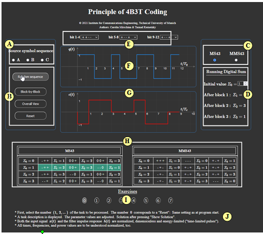
| − | '''(B)''' | + | [[File:Exercise_4B3T.png|right|600px|frame|Screenshot]] |
| + | <br><br> | ||
| + | '''(A)''' Selection of source symbol sequence: $\rm A$, $\rm B$ or $\rm C$. | ||
| + | |||
| + | '''(B)''' Program Options <br> $($random sequence, blockwise RDS calculation, total view, Reset$)$ | ||
| − | '''(C)''' | + | '''(C)''' "MS43" or "MMS43" |
| − | '''(D)''' | + | '''(D)''' Calculation of "Running Digital Sum" |
| − | '''(E)''' | + | '''(E)''' Blockwise bit change |
| − | '''(F)''' | + | '''(F)''' Graphic area for the source signal $q(t)$ |
| − | '''(G)''' | + | '''(G)''' Graphic area for the encoder signal $c(t)$ |
| − | '''(H)''' | + | '''(H)''' Total plot of values ${\it \Sigma}_0,\ {\it \Sigma}_1, \ {\it \Sigma}_2, \ {\it \Sigma}_4$ for "MS43" and "MMS43" |
| − | '''( I )''' | + | '''(I)''' Exercise selection. |
| − | '''( | + | '''(I)''' Questions and solutions |
| − | |||
<br clear=all> | <br clear=all> | ||
==About the Authors== | ==About the Authors== | ||
Latest revision as of 17:14, 26 April 2023
Open Applet in new Tab Deutsche Version Öffnen
Contents
Applet Description
The applet illustrates the principle of $\rm 4B3T$ coding. Here, in each case a block of four binary symbols is replaced by a sequence of three ternary symbols. This results in a relative code redundancy of just under $16\%$, which is used to achieve equal signal freedom.
The recoding of the sixteen possible binary blocks into the corresponding ternary blocks could in principle be done according to a fixed code table. However, to further improve the spectral characteristics of these codes, the 4B3T codes always use multiple code tables, which are selected block by block according to the "running digital sum" $(\rm RDS)$ .
In the applet, the corresponding code tables are given in the lower area, alternatively for
- the $\rm MS43$ code (from: $\rm M$onitored $\rm S$um $\rm 4$B$\rm 3$T–code), and
- the $\rm MMS43$ code (from: $\rm M$odified $\rm MS43$).
Input parameters are, besides the desired code (MS43 or MMS43), the RDS start value $\rm RDS_0$ and twelve binary source symbols $q_\nu \in \{0,\ 1\}$, either by hand, by default $($source symbol sequence $\rm A$, $\rm B$, $\rm C)$ or by random generator.
Two different modes are offered by the program:
- In the "Step" mode, the three blocks are processed successively (in each case defining the three ternary symbols, updating the RDS value and thus defining the code table for the next block.
- In the "Total" mode, only the coding results are displayed, but simultaneously for the two possible codes and in each case for all four possible RDS ;start values. The graphic and the RDS output block on the right refer to the settings made.
Theoretical Background
Classification of various coding methods
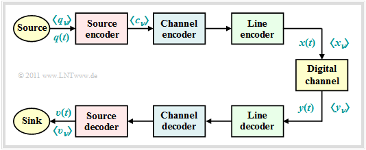
We consider the digital transmission model shown. As can be seen from this block diagram, depending on the target direction, a distinction is made between three different types of coding, each realized by the encoder at the transmitting end and the associated decoder at the receiving end:
- $\text{Source coding:}$ Removing (unnecessary) redundancy to store or transmit data as efficiently as possible ⇒ Data compression. Example: Differential pulse code modulation $\rm (DPCM)$ in image coding.
- $\text{Channel coding:}$ Targeted addition of (meaningful) redundancy, which can be used at the receiver for error detection or error detection. Main representatives: Block codes, convolutional codes, turbo codes.
- $\text{Line coding:}$ Recoding of source symbols to adapt the signal to the spectral characteristics of the channel and receiving equipment, for example to achieve a transmitted signal free of equal signals $x(t)$ for a channel with $H_{\rm K}(f = 0) = 0$ .
In the case of line codes, a further distinction is made:
- $\text{Symbol-wise coding:}$ With each incoming binary symbol $q_ν$ a multi-level (for example: ternary) code symbol $c_ν$ is generated, which also depends on the previous binary symbols. The symbol durations $T_q$ and $T_c$ are identical here. Example: Pseudo ternary codes (AMI code, duobinary code).
- $\text{Blockwise coding:}$ A block of $m_q$ binary symbols $(M_q = 2)$ is replaced by a sequence of $m_c$ higher-level symbols $(M_c > 2)$ . A characteristic of this class of codes is $T_c> T_q$. Examples include redundancy-free multi-level codes $(M_c$ is a power of two$)$ and the $\text{4B3T codes}$ considered here.
General description of 4B3T codes
The best known block code for transmission coding is the 4B3T code with the code parameters
- $$m_q = 4,\hspace{0.2cm}M_q = 2,\hspace{0.2cm}m_c = 3,\hspace{0.2cm}M_c = 3\hspace{0.05cm},$$
which was developed in the 1970s and is used, for example, in "ISDN" ("Integrated Services Digital Networks").
Such a 4B3T code has the following properties:
- Because of $m_q \cdot T_{\rm B} = m_c \cdot T$, the symbol duration $T$ of the ternary encoded signal is larger than the bit duration $T_{\rm B}$ of the binary source signal by a factor of $4/3$. This results in the favorable property that the bandwidth requirement is a quarter less than for redundancy-free binary transmission.
- The relative redundancy can be calculated with the above equation and results in $r_c \approx 16\%$. This redundancy is used in the 4B3T code to achieve DC freedom.
- The 4B3T encoder signal can thus also be transmitted over a channel (German: "Kanal" ⇒ subscript: "K") with the property $H_{\rm K}(f= 0) = 0$ without noticeable degradation.
The encoding of the sixteen possible binary blocks into the corresponding ternary blocks could in principle be performed according to a fixed code table. To further improve the spectral properties of these codes, the common 4B3T codes, viz.
- the 4B3T code according to Jessop and Waters,
- the MS43 code (from: $\rm M$onitored $\rm S$um $\rm 4$B$\rm 3$T Code),
- the FoMoT code (from: $\rm Fo$ur $\rm Mo$de $\rm T$ernary),
two or more code tables are used, the selection of which is controlled by the "running digital sum" of the amplitude coefficients. The principle is explained in the next section.
Running digital sum
After the transmission of $l$ coded blocks, the "running digital sum" with ternary amplitude coefficients $a_\nu \in \{ -1, \ 0, +1\}$:
- $${\it \Sigma}_l = \sum_{\nu = 1}^{3 \hspace{0.02cm}\cdot \hspace{0.05cm} l}\hspace{0.02cm} a_\nu \hspace{0.05cm}.$$
The selection of the table for encoding the $(l + 1)$–th block is done depending on the current ${\it \Sigma}_l$ value.
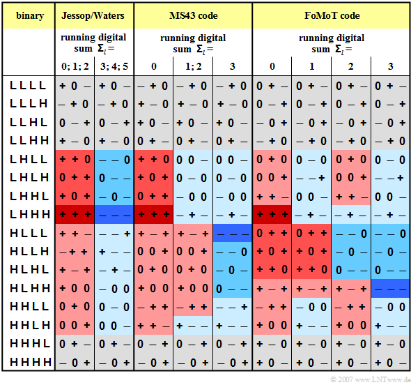
The table shows the coding rules for the three 4B3T codes mentioned above. To simplify the notation,
- "+" stands for the amplitude coefficient "+1" and
- "–" for the coefficient "–1".
You can see from the graph:
- The two code tables of the Jessop–Waters code are selected in such a way that the running digital sum ${\it \Sigma}_l$ always lies between $0$ and $5$.
- For the other two codes (MS43, FoMoT), the restriction of the running digital sum to the range $0 \le {\it \Sigma}_l \le 3$ is achieved by three resp. four alternative tables.
ACF and PSD of the 4B3T codes
The procedure for calculating the auto-correlation function $\rm (ACF)$ and the power-spectral density $\rm (PSD)$ is only outlined here in bullet points:
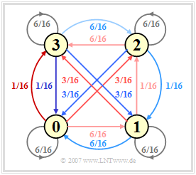
(1) The transition of the running digital sum from ${\it \Sigma}_l$ to ${\it \Sigma}_{l+1}$ is described by a homogeneous stationary first-order Markov chain with six $($Jessop–Waters$)$ or four states $($MS43, FoMoT$)$. For the FoMoT code, the Markov diagram sketched on the right applies.
(2) The values at the arrows denote the transition probabilities ${\rm Pr}({\it \Sigma}_{l+1}|{\it \Sigma}_{l})$, resulting from the respective code tables. The colors correspond to the backgrounds of the table on the last section. Due to the symmetry of the FoMoT Markov diagram, the four probabilities are all the same:
- $${\rm Pr}({\it \Sigma}_{l} = 0) = \text{...} = {\rm Pr}({\it \Sigma}_{l} = 3) = 1/4.$$
(3) The auto-correlation function $\varphi_a(\lambda) = {\rm E}\big [a_\nu \cdot a_{\nu+\lambda}\big ]$ of the amplitude coefficients can be determined from this diagram. Simpler than the analytical calculation, which requires a very large computational effort, is the simulative determination of the ACF values by computer.
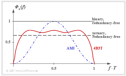
Fourier transforming the ACF yields the power-spectral density ${\it \Phi}_a(f)$ of the amplitude coefficients corresponding to the following graph from [TS87][1]. The outlined PSD was determined for the FoMoT code, whose Markov diagram is shown above. The differences between the individual 4B3T codes are not particularly pronounced. Thus, for the MS43 code ${\rm E}\big [a_\nu^2 \big ] \approx 0.65$ and for the other two 4B3T codes (Jessop/Waters, MS43) ${\rm E}\big [a_\nu^2 \big ] \approx 0.69$.
The statements of this graph can be summarized as follows:
- The graph shows the power-spectral density ${\it \Phi}_a(f)$ of the amplitude coefficients $a_\nu$ of the 4B3T code ⇒ red curve.
- The PSD ${\it \Phi}_s(f)$ including the transmission pulse is obtained by multiplying by $1/T \cdot |G_s(f)|^2$ ⇒ ${\it \Phi}_a(f)$ must be multiplied by a $\rm sinc^2$ function, if $g_s(t)$ describes a rectangular pulse.
- Redundancy-free binary or ternary coding results in a constant ${\it \Phi}_a(f)$ in each case, the magnitude of which depends on the number $M$ of levels (different signal power).
- In contrast, the 4B3T power-spectral density has zeros at $f = 0$ and multiples of $f = 1/T$.
- The zero point at $f = 0$ has the advantage that the 4B3T signal can also be transmitted without major losses via a so-called "telephone channel", which is not suitable for a DC signal due to transformers.
- The zero point at $f = 1/T$ has the disadvantage that this makes clock recovery at the receiver more difficult. Outside of these zeros, the 4B3T codes have a flatter ${\it \Phi}_a(f)$ than the "AMI code" discussed in the next chapter (blue curve), which is advantageous.
- The reason for the flatter PSD curve at medium frequencies as well as the steeper drop towards the zeros is that for the 4B3T codes up to five $+1$ coefficients (resp. $-1$ coefficients) can follow each other. With the AMI code, these symbols occur only in isolation.
Exercises
- First, select the number $(1,\ 2, \text{...} \ )$ of the task to be processed. The number $0$ corresponds to a "Reset": Same setting as at program start.
- A task description is displayed. The parameter values are adjusted. Solution after pressing "Show Solution".
- Both the input signal $x(t)$ and the filter impulse response $h(t)$ are normalized, dimensionless and energy-limited ("time-limited pulses").
- All times, frequencies, and power values are to be understood normalized, too.
(1) Illustrate the 4B3T coding of the source symbol sequence $\rm A$ ⇒ $\langle q_\nu \rangle = \langle 0, 1, 0, 1; \ 1, 0, 1, 1; \ 0, 1, 1, 0 \rangle $ according to the $\rm MS43$ code ("Block–by–Block").
Let the RDS initial value be ${\it \Sigma}_0= 0$. Note: The source symbol sequence is already divided by semicolons into subsequences of four bits each.
- Starting from the RDS initial value ${\it \Sigma}_0= 0$ you recognize the following coding of the first four bits (first block): $(0, 1, 0, 1)\ \rightarrow\ (+,\ 0 ,\ +) $ ⇒ ${\it \Sigma}_1= 2.$
- For the next four bits (second block), now assume ${\it \Sigma}_1= 2$ $(1, 0, 1, 1)\ \rightarrow\ (+,\ 0 ,\ 0) $ ⇒ ${\it \Sigma}_2= 3.$
- The encoding of bits 9 to 12 (third block) results: ${\it \Sigma}_2= 3$ to $(0, 1, 1, 0,)\ \rightarrow\ (-,\ 0 ,\ 0) $ ⇒ ${\it \Sigma}_3= 2.$
(2) Repeat this experiment with the other possible RDS initial values ${\it \Sigma}_0= 1$, ${\it \Sigma}_0= 2$ and ${\it \Sigma}_0= 3.$ How do the coding results differ?
- ${\it \Sigma}_0= 1$: $(0, 1, 0, 1)\ \rightarrow\ (0,\ - ,\ 0) $ ⇒ ${\it \Sigma}_1= 0$: $(1, 0, 1, 1)\ \rightarrow\ (+,\ 0 ,\ 0) $ ⇒ ${\it \Sigma}_2= 1$: $(0, 1, 1, 0)\ \rightarrow\ (-,\ 0 ,\ 0) $ ⇒ ${\it \Sigma}_3= 0.$
- ${\it \Sigma}_0= 2$: $(0, 1, 0, 1)\ \rightarrow\ (0,\ - ,\ 0) $ ⇒ ${\it \Sigma}_1= 1$: $(1, 0, 1, 1)\ \rightarrow\ (+,\ 0 ,\ 0) $ ⇒ ${\it \Sigma}_2= 2$: $(0, 1, 1, 0)\ \rightarrow\ (-,\ 0 ,\ 0) $ ⇒ ${\it \Sigma}_3= 1.$
- ${\it \Sigma}_0= 3$: $(0, 1, 0, 1)\ \rightarrow\ (0,\ - ,\ 0) $ ⇒ ${\it \Sigma}_1= 2$: $(1, 0, 1, 1)\ \rightarrow\ (+,\ 0 ,\ 0) $ ⇒ ${\it \Sigma}_2= 3$: $(0, 1, 1, 0)\ \rightarrow\ (-,\ 0 ,\ 0) $ ⇒ ${\it \Sigma}_3= 2.$
(3) How many different code tables does the $\rm MS43$ code use?
- From the previous experiments, we can see that the MS43 code uses at least two tables, switching between them according to the current RDS value.
- From the table given in the applet, it can be seen that three tables are actually used. The entries for ${\it \Sigma}_l= 1$ and ${\it \Sigma}_l= 2$ are in fact identical.
(4) Interpret the results of 4B3T coding for the source symbol sequence $\rm B$ ⇒ $\langle q_\nu \rangle = \langle 1, 1, 1, 0; \ 0, 0, 1, 0; \ 1, 1, 1 \rangle $ and the MS43 code.
- For this source symbol sequence, the RDS value is not changed. For each starting value $(0$, $1$, $2$ and $3)$ holds ${\it \Sigma}_0 = {\it \Sigma}_1 ={\it \Sigma}_2 ={\it \Sigma}_3 $, for example:
- ${\it \Sigma}_0= 1$: $(1, 1, 1, 0)\ \rightarrow\ (0,\ - ,\ +) $ ⇒ ${\it \Sigma}_1= 1$: $(0, 0, 1, 0)\ \rightarrow\ (+,\ 0 ,\ -) $ ⇒ ${\it \Sigma}_2= 1$: $(1, 1, 1, 1)\ \rightarrow\ (-,\ 0 ,\ +) $ ⇒ ${\it \Sigma}_3= 1.$
- The reason for this is that with this source symbol sequence, each ternary–triple contains exactly one "plus" and one "minus" after encoding.
(5) In contrast, how many different code tables does the modified MS43 code ⇒ $\rm MMS43$ use?
- It can be seen from the table given in the applet that in the modified MS43 code all four tables are in fact different.
- The entries for ${\it \Sigma}_l= 1$ and ${\it \Sigma}_l= 2$ are indeed largely the same. They differ only for the binary sequences $(0, 1, 1, 0)$ and $(1, 0, 1, 0)$.
- The $\rm MMS43$ code is used with $\rm ISDN$ ("Integrated Services Digital Network") on the local loop $(U_{K0}$ interface$)$.
- We do not know why the original MS43 code was modified during standardization. We suspect a slightly more favorable power density spectrum.
(6) Compare the $\rm MS43$ and $\rm MMS43$ results for the source symbol sequences $\rm A$ and $\rm B$ and any RDS initial values. Select "Overall View".
- For source symbol sequence $\rm A$ there are two different $\rm MS43$ code symbol sequences and three different $\rm MMS43$ code symbol sequences.
- For the source symbol sequence $\rm B$ the $\rm MS43$ code symbol sequences are the same for all possible RDS initial values. For $\rm MMS43$: two different coding results.
(7) Interpret the results for the sequence $\rm C$ ⇒ $\langle q_\nu \rangle = \langle 0, 1, 1, 0; \ 0, 1, 1, 0; \ 0, 1, 1, 0 \rangle $ for both codes and all RDS initial values. Select "Overall View".
- The four input bits of each block are $(0,\ 1,\ 1,\ 0)$. With $\rm MS43$ these are replaced by $(0,\ +,\ +)$, if ${\it \Sigma}_l=0$; resp. $(-,\ 0,\ 0)$, if ${\it \Sigma}_l\ne0$.
- In the $\rm MMS43$, however, these are replaced by $(-,\ +,\ +)$, if ${\it \Sigma}_l\le 1$; resp. $(-,\ -,\ +)$, if ${\it \Sigma}_l\ge 2$. Only if you have enough time to spare:
- Try to make sense of this modification from $\rm MS43$ to $\rm MMS43$. Our LNTww team did not succeed.
Applet Manual
(A) Selection of source symbol sequence: $\rm A$, $\rm B$ or $\rm C$.
(B) Program Options
$($random sequence, blockwise RDS calculation, total view, Reset$)$
(C) "MS43" or "MMS43"
(D) Calculation of "Running Digital Sum"
(E) Blockwise bit change
(F) Graphic area for the source signal $q(t)$
(G) Graphic area for the encoder signal $c(t)$
(H) Total plot of values ${\it \Sigma}_0,\ {\it \Sigma}_1, \ {\it \Sigma}_2, \ {\it \Sigma}_4$ for "MS43" and "MMS43"
(I) Exercise selection.
(I) Questions and solutions
About the Authors
This interactive calculation tool was designed and implemented at the Institute for Communications Engineering at the Technical University of Munich.
- The first version was created in 2010 by Stefan Müller as part of his bachelor thesis with “FlashMX – Actionscript” (Supervisor: Günter Söder).
- Last revision and English version 2020/2021 by Carolin Mirschina in the context of a working student activity.
The conversion of this applet to HTML 5 was financially supported by Studienzuschüsse ("study grants") of the TUM Faculty EI. We thank.
Once again: Open Applet in new Tab
Open Applet in new Tab Deutsche Version Öffnen
- ↑ Tröndle, K.; Söder, G.: Optimization of Digital Transmission Systems. Boston – London: Artech House, 1987, ISBN: 0-89006-225-0.
