Aufgaben:Exercise 4.16: Eigenvalues and Eigenvectors: Difference between revisions
Join split $$ formula lines for correct rendering |
Fix interlanguage link: resolve redirect chain |
||
| (2 intermediate revisions by the same user not shown) | |||
| Line 103: | Line 103: | ||
The eigenvectors are obtained by substituting the eigenvalues $\lambda_1$ and $\lambda_2$ into the correlation matrix: | The eigenvectors are obtained by substituting the eigenvalues $\lambda_1$ and $\lambda_2$ into the correlation matrix: | ||
:$$\left[ \begin{array}{cc} | :$$\left[ \begin{array}{cc}1- (1+\rho) & \rho \\\rho & 1- (1+\rho)\end{array} \right]\cdot{\boldsymbol{\eta_1}} = \left[ \begin{array}{cc}-\rho & \rho \\\rho & -\rho\end{array} \right]\cdot \left[ \begin{array}{c}\eta_{11} \\\eta_{12}\end{array} \right]=0$$:$$\Rightarrow\hspace{0.3cm}-\rho \cdot \eta_{11} + \rho \cdot\eta_{12} = 0\hspace{0.3cm}\Rightarrow\hspace{0.3cm}\eta_{11}={\rm const} \cdot\eta_{12}\hspace{0.3cm}\Rightarrow\hspace{0.3cm}{\boldsymbol{\eta_1}}={\rm const}\cdot \left[ \begin{array}{c}1 \\1\end{array} \right];$$:$$\left[ \begin{array}{cc}1- (1-\rho) & \rho \\\rho & 1- (1-\rho)\end{array} \right]\cdot{\boldsymbol{\eta_2}} = \left[ \begin{array}{cc}\rho & \rho \\\rho & \rho\end{array} \right]\cdot \left[ \begin{array}{c}\eta_{21} \\\eta_{22}\end{array} \right]=0$$:$$\Rightarrow\hspace{0.3cm}\rho \cdot \eta_{21} + \rho \cdot\eta_{22} = 0\hspace{0.3cm}\Rightarrow\hspace{0.3cm}\eta_{21}=-{\rm const} \cdot\eta_{22}\hspace{0.3cm}\Rightarrow\hspace{0.3cm}{\boldsymbol{\eta_2}}={\rm const}\cdot \left[ \begin{array}{c}-1 \\1\end{array} \right].$$[[File:P_ID676__Sto_A_4_16_d.png|right|frame|Rotate the coordinate system]]Putting this into the "orthonormal form", the following holds::$${\boldsymbol{\eta_1}}= \frac{1}{\sqrt{2}}\cdot \left[\begin{array}{c}1 \\1\end{array} \right],\hspace{0.5cm}{\boldsymbol{\eta_2}}= \frac{1}{\sqrt{2}}\cdot \left[\begin{array}{c}-1 \\1\end{array} \right].$$ | ||
1- (1+\rho) & \rho \\ | |||
\rho & 1- (1+\rho) | |||
\end{array} \right]\cdot{\boldsymbol{\eta_1}} = \left[ \begin{array}{cc} | |||
-\rho & \rho \\ | |||
\rho & -\rho | |||
\end{array} \right]\cdot \left[ \begin{array}{c} | |||
\eta_{11} \\ | |||
\eta_{12} | |||
\end{array} \right]=0$$:$$\Rightarrow\hspace{0.3cm}-\rho \cdot \eta_{11} + \rho \cdot | |||
\eta_{12} = 0\hspace{0.3cm}\Rightarrow\hspace{0.3cm}\eta_{11}= | |||
{\rm const} \cdot | |||
\eta_{12}\hspace{0.3cm}\Rightarrow\hspace{0.3cm}{\boldsymbol{\eta_1}}= | |||
{\rm const}\cdot \left[ \begin{array}{c} | |||
1 \\ | |||
1 | |||
\end{array} \right];$$:$$\left[ \begin{array}{cc} | |||
1- (1-\rho) & \rho \\ | |||
\rho & 1- (1-\rho) | |||
\end{array} \right]\cdot{\boldsymbol{\eta_2}} = \left[ \begin{array}{cc} | |||
\rho & \rho \\ | |||
\rho & \rho | |||
\end{array} \right]\cdot \left[ \begin{array}{c} | |||
\eta_{21} \\ | |||
\eta_{22} | |||
\end{array} \right]=0$$:$$\Rightarrow\hspace{0.3cm}\rho \cdot \eta_{21} + \rho \cdot | |||
\eta_{22} = 0\hspace{0.3cm}\Rightarrow\hspace{0.3cm}\eta_{21}= | |||
-{\rm const} \cdot | |||
\eta_{22}\hspace{0.3cm}\Rightarrow\hspace{0.3cm}{\boldsymbol{\eta_2}}= | |||
{\rm const}\cdot \left[ \begin{array}{c} | |||
-1 \\ | |||
1 | |||
\end{array} \right].$$[[File:P_ID676__Sto_A_4_16_d.png|right|frame|Rotate the coordinate system]]Putting this into the "orthonormal form", the following holds::$${\boldsymbol{\eta_1}}= \frac{1}{\sqrt{2}}\cdot \left[ | |||
\begin{array}{c} | |||
1 \\ | |||
1 | |||
\end{array} \right],\hspace{0.5cm} | |||
{\boldsymbol{\eta_2}}= \frac{1}{\sqrt{2}}\cdot \left[ | |||
\begin{array}{c} | |||
-1 \\ | |||
1 | |||
\end{array} \right].$$ | |||
The sketch illustrates the result: | The sketch illustrates the result: | ||
| Line 172: | Line 131: | ||
[[File:P_ID677__Sto_A_4_16_g.png|right|frame|Best possible decorrelation]] | [[File:P_ID677__Sto_A_4_16_g.png|right|frame|Best possible decorrelation]] | ||
The same result is obtained using the eigenvector: | The same result is obtained using the eigenvector: | ||
:$$\left[ \begin{array}{cc} | :$$\left[ \begin{array}{cc}4-5 & 2 \\2 & 1-5\end{array} \right]\cdot \left[ \begin{array}{c}\zeta_{11} \\\zeta_{12}\end{array}\right]=0 \hspace{0.3cm}\Rightarrow\hspace{0.3cm}-\zeta_{11}=2\zeta_{12}=0\hspace{0.3cm}\Rightarrow\hspace{0.3cm}\zeta_{12}={\zeta_{11}}/{2}$$:$$\Rightarrow\hspace{0.3cm}\alpha = \arctan({\zeta_{12}}/{\zeta_{11}}) = \arctan(0.5) \hspace{0.15cm}\underline{= 26.56^\circ}.$$ | ||
4-5 & 2 \\ | |||
2 & 1-5 | |||
\end{array} \right]\cdot \left[ \begin{array}{c} | |||
\zeta_{11} \\ | |||
\zeta_{12} | |||
\end{array} | |||
\right]=0 \hspace{0.3cm} | |||
\Rightarrow\hspace{0.3cm}-\zeta_{11}= | |||
2\zeta_{12}=0\hspace{0.3cm}\Rightarrow\hspace{0.3cm}\zeta_{12}={\zeta_{11}}/{2}$$:$$\Rightarrow\hspace{0.3cm}\alpha = \arctan | |||
({\zeta_{12}}/{\zeta_{11}}) = \arctan(0.5) \hspace{0.15cm}\underline{= 26.56^\circ}.$$ | |||
The accompanying sketch shows the joint PDF of the random variable $\mathbf{z}$: | The accompanying sketch shows the joint PDF of the random variable $\mathbf{z}$: | ||
| Line 194: | Line 143: | ||
[[Category:Theory of Stochastic Signals: Exercises|^4.7 N-dimensionale Zufallsgrößen^]] | [[Category:Theory of Stochastic Signals: Exercises|^4.7 N-dimensionale Zufallsgrößen^]] | ||
[[de:Aufgaben:4. | [[de:Aufgaben:Aufgabe 4.16: Eigenwerte und Eigenvektoren]] | ||
Latest revision as of 17:58, 16 March 2026

Although the description of Gaussian random variables using vectors and matrices is actually only necessary and makes sense for more than $N = 2$ dimensions, here we restrict ourselves to the special case of two-dimensional random variables for simplicity.
In the graph above, the general correlation matrix $\mathbf{K_x}$ of the two-dimensional random variable $\mathbf{x} = (x_1, x_2)^{\rm T}$ is given, where $\sigma_1^2$ and $\sigma_2^2$ describe the variances of the individual components. $\rho$ denotes the correlation coefficient between the two components.
The random variables $\mathbf{y}$ and $\mathbf{z}$ give two special cases of $\mathbf{x}$ whose process parameters are to be determined from the correlation matrices $\mathbf{K_y}$ and $\mathbf{K_z}$ respectively.
Hints:
- The exercise belongs to the chapter Generalization to N-Dimensional Random Variables.
- Some basics on the application of vectors and matrices can be found on the pages Determinant of a Matrix and Inverse of a Matrix .
- According to the page "Contour lines for correlated random variables" the angle $\alpha$ between the old and the new system is given by the following equation:
- $$\alpha = {1}/{2}\cdot \arctan (2 \cdot\rho \cdot\frac{\sigma_1\cdot\sigma_2}{\sigma_1^2 -\sigma_2^2}).$$
- In particular, note:
- A $2×2$-covariance matrix has two real eigenvalues $\lambda_1$ and $\lambda_2$.
- These two eigenvalues determine two eigenvectors $\xi_1$ and $\xi_2$.
- These span a new coordinate system in the direction of the principal axes of the old system.
Questions
Solution
- $\mathbf{K_y}$ is indeed the most general correlation matrix of a two-dimensional random variable with $\sigma_1 = \sigma_2 = \sigma$.
- The parameter $\rho$ specifies the correlation coefficient. This can take all values between $\pm 1$ including these marginal values.
(2) In this case, the governing equation is:
- $${\rm det}\left[ \begin{array}{cc}1- \lambda & 0 \\0 & 1- \lambda\end{array} \right] = 0 \hspace{0.3cm}\Rightarrow \hspace{0.3cm}(1- \lambda)^2 = 0\hspace{0.3cm}\Rightarrow\hspace{0.3cm} \hspace{0.15cm}\underline{\lambda_{1/2} =1}.$$
(3) With positive $\rho$ the governing equation of the eigenvalues is:
- $$(1- \lambda)^2 -\rho^2 = 0\hspace{0.5cm}\Rightarrow\hspace{0.5cm}\lambda^2 - 2\lambda + 1 - \rho^2 =0\hspace{0.5cm}\Rightarrow\hspace{0.5cm}\lambda_{1/2} =1 \pm \rho.$$
- For $\rho= 0.5$ one gets $\underline{\lambda_{1} =1.5}$ and $\underline{\lambda_{2} =0.5}$.
- By the way, the equation holds in the whole domain of definition $-1 \le \rho \le +1$.
- For $\rho = 0$ ⇒ $\lambda_1 = \lambda_2 = +1$ ⇒ see subtask (2).
- For $\rho = \pm 1$ ⇒ $\lambda_1 = 2$ and $\lambda_2 = 0$.
(4) Correct are the proposed solutions 1 and 2.
The eigenvectors are obtained by substituting the eigenvalues $\lambda_1$ and $\lambda_2$ into the correlation matrix:
- $$\left[ \begin{array}{cc}1- (1+\rho) & \rho \\\rho & 1- (1+\rho)\end{array} \right]\cdot{\boldsymbol{\eta_1}} = \left[ \begin{array}{cc}-\rho & \rho \\\rho & -\rho\end{array} \right]\cdot \left[ \begin{array}{c}\eta_{11} \\\eta_{12}\end{array} \right]=0$$:$$\Rightarrow\hspace{0.3cm}-\rho \cdot \eta_{11} + \rho \cdot\eta_{12} = 0\hspace{0.3cm}\Rightarrow\hspace{0.3cm}\eta_{11}={\rm const} \cdot\eta_{12}\hspace{0.3cm}\Rightarrow\hspace{0.3cm}{\boldsymbol{\eta_1}}={\rm const}\cdot \left[ \begin{array}{c}1 \\1\end{array} \right];$$:$$\left[ \begin{array}{cc}1- (1-\rho) & \rho \\\rho & 1- (1-\rho)\end{array} \right]\cdot{\boldsymbol{\eta_2}} = \left[ \begin{array}{cc}\rho & \rho \\\rho & \rho\end{array} \right]\cdot \left[ \begin{array}{c}\eta_{21} \\\eta_{22}\end{array} \right]=0$$:$$\Rightarrow\hspace{0.3cm}\rho \cdot \eta_{21} + \rho \cdot\eta_{22} = 0\hspace{0.3cm}\Rightarrow\hspace{0.3cm}\eta_{21}=-{\rm const} \cdot\eta_{22}\hspace{0.3cm}\Rightarrow\hspace{0.3cm}{\boldsymbol{\eta_2}}={\rm const}\cdot \left[ \begin{array}{c}-1 \\1\end{array} \right].$$
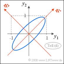
Rotate the coordinate system

The sketch illustrates the result:
- The coordinate system defined by $\mathbf{\eta_1}$ and $\mathbf{\eta_2}$ is actually in the direction of the main axes of the original system.
- With $\sigma_1 = \sigma_2$ almost always results $($exception: $\rho= 0)$ the rotation angle $\alpha = 45^\circ$.
- This also follows from the equation given in the theory section:
- $$\alpha = {1}/{2}\cdot \arctan (2 \cdot\rho \cdot\frac{\sigma_1\cdot\sigma_2}{\sigma_1^2 -\sigma_2^2})={1}/{2}\cdot \arctan(\infty)\hspace{0.3cm}\rightarrow\hspace{0.3cm}\alpha = 45^\circ.$$
- The eigenvalues $\lambda_1$ and $\lambda_2$ do not denote the standard deviations with respect to the new axes, but the variances.
(5) By comparing the matrices $\mathbf{K_x}$ and $\mathbf{K_z}$ we get.
- $\sigma_{1}\hspace{0.15cm}\underline{ =2}$,
- $\sigma_{2}\hspace{0.15cm}\underline{ =1}$,
- $\rho = 2/(\sigma_{1} \cdot \sigma_{2})\hspace{0.15cm}\underline{ =1}$.
(6) According to the now familiar scheme:
- $$(4- \lambda) \cdot (1- \lambda) -4 = 0\hspace{0.3cm}\Rightarrow\hspace{0.3cm}\lambda^2 - 5\lambda =0\hspace{0.3cm}\Rightarrow\hspace{0.3cm}\hspace{0.15cm}\underline{\lambda_{1}=5,\hspace{0.1cm} \lambda_{2} =0}.$$
(7) According to the equation given on the specification sheet:
- $$\alpha ={1}/{2}\cdot \arctan (2 \cdot 1 \cdot \frac{2 \cdot1}{2^2 -1^2})= {1}/{2}\cdot \arctan ({4}/{3}) =26.56^\circ.$$

The same result is obtained using the eigenvector:
- $$\left[ \begin{array}{cc}4-5 & 2 \\2 & 1-5\end{array} \right]\cdot \left[ \begin{array}{c}\zeta_{11} \\\zeta_{12}\end{array}\right]=0 \hspace{0.3cm}\Rightarrow\hspace{0.3cm}-\zeta_{11}=2\zeta_{12}=0\hspace{0.3cm}\Rightarrow\hspace{0.3cm}\zeta_{12}={\zeta_{11}}/{2}$$:$$\Rightarrow\hspace{0.3cm}\alpha = \arctan({\zeta_{12}}/{\zeta_{11}}) = \arctan(0.5) \hspace{0.15cm}\underline{= 26.56^\circ}.$$
The accompanying sketch shows the joint PDF of the random variable $\mathbf{z}$:
- Because of $\rho = 1$ all values lie on the correlation line with coordinates $z_1$ and $z_2 = z_1/2$.
- By rotating by the angle $\alpha = \arctan(0.5) = 26.56^\circ$ a new coordinate system is formed.
- The variance along the axis $\mathbf{\zeta_1}$ is $\lambda_1 = 5$ $($standard deviation $\sigma_1 = \sqrt{5} = 2.236)$,
- while in the direction orthogonal to it, the random variable $\mathbf{\zeta_2}$ is not extended $(\lambda_2 = \sigma_2 = 0)$.
