Die Seite wurde neu angelegt: „ {{quiz-Header|Buchseite=Stochastische Signaltheorie/Zweidimensionale Gaußsche Zufallsgrößen }} right| :Wir betrachten…“
:Wir betrachten zweidimensionale Zufallsgrößen, wobei beide Komponenten stets als mittelwertfrei vorausgesetzt werden. Die 2D-WDF der Zufallsgröße (<i>u</i>, <i>υ</i>) lautet:
We consider two-dimensional random variables, where both components are always assumed to be mean-free.
:Die Werte des Gaußschen Fehlerintegrals <i>ϕ</i>(<i>x</i>) sowie der Komplementärfunktion Q(<i>x</i>) = <i>ϕ</i>(–<i>x</i>) = 1 – <i>ϕ</i>(<i>x</i>) können Sie der nebenstehenden Tabelle entnehmen.
:<br><br><br><br><br>
:<b>Hinweis:</b> Die Aufgabe bezieht sich auf den Lehrstoff von Kapitel 3.5 und Kapitel 4.2.
:Die hier behandelte Thematik ist in zwei Lernvideos zusammengefasst:
===Fragebogen===
Hints:
*The exercise belongs to the chapter [[Theory_of_Stochastic_Signals/Two-Dimensional_Gaussian_Random_Variables|»Two-dimensional Gaussian Random Variables«]].
*Reference is also made to the chapter [[Theory_of_Stochastic_Signals/Gaussian_Distributed_Random_Variables|»Gaussian distributed random variables«]].
===Questions===
<quiz display=simple>
<quiz display=simple>
{Welche der Aussagen gelten hinsichtlich der Zufallsgröße (<i>u</i>, <i>υ</i>)?
{Which of the statements are true with respect to the two-dimensional random variable $(u, v)$ ?
|type="[]"}
|type="[]"}
+ Die Zufallsgrößen <i>u</i> und <i>υ</i> sind unkorreliert.
+ The random variables $u$ and $v$ are uncorrelated.
+ Die Zufallsgrößen <i>u</i> und <i>υ</i> sind statistisch unabhängig.
+ The random variables $u$ and $v$ are statistically independent.
{Berechnen Sie die beiden Streuungen <i>σ<sub>u</sub></i> und <i>σ<sub>υ</sub></i>. Geben Sie zur Kontrolle den Quotienten der beiden Streuungen ein.
{Calculate the two standard deviations $\sigma_u$ and $\sigma_v$. Enter the quotient of the two standard deviations as a check.
|type="{}"}
|type="{}"}
$\sigma_u/\sigma_v$ = { 0.5 3% }
$\sigma_u/\sigma_v \ = \ $ { 0.5 3% }
{Berechnen Sie die Wahrscheinlichkeit, dass <i>u</i> kleiner als 1 ist.
{Calculate the probability that $u$ is less than $1$.
|type="{}"}
|type="{}"}
$Pr(u < 1)$ = { 0.9772 3% }
${\rm Pr}(u < 1)\ = \ $ { 0.9772 3% }
{Berechnen Sie die Wahrscheinlichkeit, dass die Zufallsgröße <i>u</i> kleiner als 1 und gleichzeitig die Zufallsgröße <i>υ</i> größer als 1 ist.
{Calculate the probability that the random variable $u$ is less than $1$ and at the same time the random variable $v$ is greater than $1$.
{Welche der Aussagen sind für die 2D-Zufallsgröße (<i>x</i>, <i>y</i>) zutreffend?
{Which of the statements are true for the two-dimensional random variable $(x, y)$?
|type="[]"}
|type="[]"}
+ Die 2D-WDF <i>f<sub>xy</sub></i>(<i>x</i>, <i>y</i>) ist außerhalb der Geraden <i>y</i> = 2<i>x</i> stets 0.
+ The joint probability density function $f_{xy}(x, y)$ is always zero outside the straight line $y = 2x$.
- Für alle Wertepaare auf der Geraden <i>y</i> = 2<i>x</i> gilt <i>f<sub>xy</sub></i>(<i>x</i>, <i>y</i>) = 0.5.
- For all pairs of values on the straight line $y = 2x$ holds: $f_{xy}(x, y)= 0.5$.
+ Bezüglich der Rand-WDF gilt <i>f<sub>x</sub></i>(<i>x</i>) = <i>f<sub>u</sub></i>(<i>u</i>) bzw. <i>f<sub>y</sub></i>(<i>y</i>) = <i>f<sub>υ</sub></i>(<i>υ</i>).
+ With respect to the edge PDFs: $f_{x}(x) = f_{u}(u)$ and $f_{y}(y) = f_{v}(v)$ holds.
{Berechnen Sie die Wahrscheinlichkeit, dass <i>x</i> kleiner als 1 ist.
{Calculate the probability that $x$ is less than $1$.
|type="{}"}
|type="{}"}
$Pr(x < 1)$ = { 0.9772 3% }
${\rm Pr}(x < 1)\ = \ $ { 0.9772 3% }
{Berechnen Sie nun die Wahrscheinlichkeit, dass die Zufallsgröße <i>x</i> kleiner als 1 und gleichzeitig <i>y</i> größer als 1 ist.
{Now calculate the probability that the random variable $x$ is less than $1$ and at the same time the random variable $y$ is greater than $1$.
:so erkennt man, dass im Exponenten kein Term mit <i>u</i> · <i>υ</i> auftritt, was nur bei <i>ρ<sub>uυ</sub></i> = 0 möglich ist. Dies bedeutet aber, dass <i>u</i> und <i>υ</i> unkorreliert sind. Bei Gaußschen Zufallsgrößen folgt aus der Unkorreliertheit aber auch stets die statistische Unabhängigkeit.
:so it can be seen that no term with $u \cdot v$ occurs in the exponent, which is only possible with $\rho_{uv} = 0$.
*But this means that $u$ and $v$ are uncorrelated.
*For Gaussian random variables, however, statistical independence always follows from uncorrelatedness.
:Durch Koeffizientenvergleich erhält man <i>σ<sub>u</sub></i> = 0.5 und <i>σ<sub>υ</sub></i> = 1. Der Quotient ist somit <i>σ<sub>u</sub></i>/<i>σ<sub>υ</sub></i> <u>= 0.5</u>.
:<b>3.</b> Da <i>u</i> eine kontinuierliche Zufallsgröße ist, gilt:
'''(2)''' With statistical independence holds:
:$$\rm Pr(\it u < \rm 1) = \rm Pr(\it u \le \rm 1) =\it F_u(\rm 1). $$
*The quotient is thus $\sigma_u/\sigma_v\hspace{0.15cm}\underline{=0.5}$.
:<b>4.</b> Aufgrund der statistischen Unabhängigkeit zwischen <i>u</i> und <i>υ</i> gilt:
:$$\rm Pr((\it u < \rm 1) \cap (\it v > \rm 1)) = \rm Pr(\it u < \rm 1)\cdot \rm Pr(\it v > \rm 1).$$
:Die Wahrscheinlichkeit Pr(<i>u</i> < 1) =0.9772 wurde bereits berechnet. Für die zweite Wahrscheinlichkeit Pr(<i>υ</i> > 1) gilt aus Symmetriegründen:
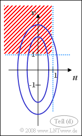
:Die obige Skizze verdeutlicht die vorgegebene Konstellation. Die Höhenlinien der WDF (blau) sind wegen <i>σ<sub>υ</sub></i> > <i>σ<sub>u</sub></i> in vertikaler Richtung gestreckte Ellipsen. Rot schraffiert eingezeichnet ist das Gebiet, dessen Wahrscheinlichkeit in dieser Teilaufgabe berechnet werden sollte.
'''(3)''' Because $u$ is a continuous random variable:
[[File:P_ID266__Sto_A_4_4_e.png|right|]]
:$$\rm Pr(\it u < \rm 1) = \rm Pr(\it u \le \rm 1) =\it F_u\rm (1). $$
:<b>5.</b> Wegen <i>ρ<sub>xy</sub></i> = 1 besteht ein deterministischer Zusammenhang zwischen <i>x</i> und <i>y</i> ⇒ alle Werte liegen auf der Geraden <i>y</i> = <i>K</i> · <i>x</i>. Aufgrund der Streuungen <i>σ<sub>x</sub></i> = 0.5 und <i>σ<sub>y</sub></i> = 1 gilt <i>K</i> = 2.
*With the mean $m_u = 0$ and the standard deviation $\sigma_u = 0.5$ we get:
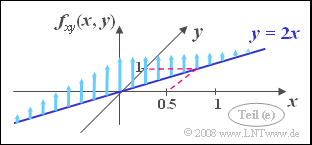
:Auf dieser Geraden <i>y</i> = 2<i>x</i> sind alle WDF-Werte unendlich groß. Das bedeutet: Die 2D-WDF ist hier eine „Diracwand”.
:Wie aus der Skizze hervorgeht, sind die WDF–Werte auf der Geraden <i>y</i> = 2<i>x</i>, die gleichzeitig die Korrelationsgerade darstellt, gaußverteilt. Auch die beiden Randwahrscheinlichkeitsdichten sind hier Gaußfunktionen, jeweils mit dem Mittelwert 0. Da <i>σ<sub>x</sub></i> = <i>σ<sub>u</sub></i> und <i>σ<sub>y</sub></i> = <i>σ<sub>υ</sub></i> ist, gilt auch:
[[File:P_ID265__Sto_A_4_4_d.png|right|frame|$\rm Pr\big[(\it u < \rm 1) \cap (\it v > \rm 1)\big]$]]
:<b>6.</b> Da die WDF der Zufallsgröße <i>x</i> identisch mit der WDF <i>f<sub>u</sub></i>(<i>u</i>) ist, ergibt sich auch genau die gleiche Wahrscheinlichkeit wie in der Teilaufgabe (c) berechnet:
The sketch on the right illustrates the given constellation:
[[File:P_ID274__Sto_A_4_4_g.png|right|]]
*The PDF contour lines (blue) are stretched ellipses due to $\sigma_v > \sigma_u$ in vertical direction.
:$$\rm Pr(\it x < \rm 1) \hspace{0.15cm}\underline{ = \rm 0.9772}.$$
*Drawn in red (shading) is the area whose probability should be calculated in this subtask.
[[File:P_ID266__Sto_A_4_4_e.png|right|frame|"Dirac wall" on the correlation line]]
'''(5)''' Correct are <u>the first and the third suggested solutions</u>:
*Because $\rho_{xy} = 1$ there is a deterministic correlation between $x$ and $y$
:⇒ All values lie on the straight line $y =K \cdot x$.
*Because of the standard deviations $\sigma_x = 0.5$ and $\sigma_y = 1$ it holds $K = 2$.
*On this straight line $y = 2x$ ⇒ all PDF values are infinitely large.
*This means: The joint PDF is here a "Dirac wall".
*As you can see from the sketch, the PDF values are Gaussian distributed on the straight line $y = 2x$.
*The two marginal probability densities are also Gaussian functions, each with zero mean.
:<b>7.</b> Das Zufallsereignis „<i>y</i> > 1“ ist identisch mit dem Ereignis „<i>x</i> > 0.5“. Damit ist die gesuchte Wahrscheinlichkeit gleich
'''(6)''' Since the PDF of the random variable $x$ is identical to the PDF $f_u(u)$, it also results in exactly the same probability as calculated in the subtask '''(3)''':
:$$\rm Pr(\it x < \rm 1) \hspace{0.15cm}\underline{ = \rm 0.9772}.$$
:<br><br>
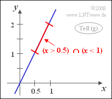
'''(7)''' The random event $y > 1$ is identical to the event $x > 0.5$.
(6) Since the PDF of the random variable $x$ is identical to the PDF $f_u(u)$, it also results in exactly the same probability as calculated in the subtask (3):
$$\rm Pr(\it x < \rm 1) \hspace{0.15cm}\underline{ = \rm 0.9772}.$$
(7) The random event $y > 1$ is identical to the event $x > 0.5$.